
1Start here
What FlavoRotor is, which variables the system controls and which plant responses it measures.
1.1Research overview
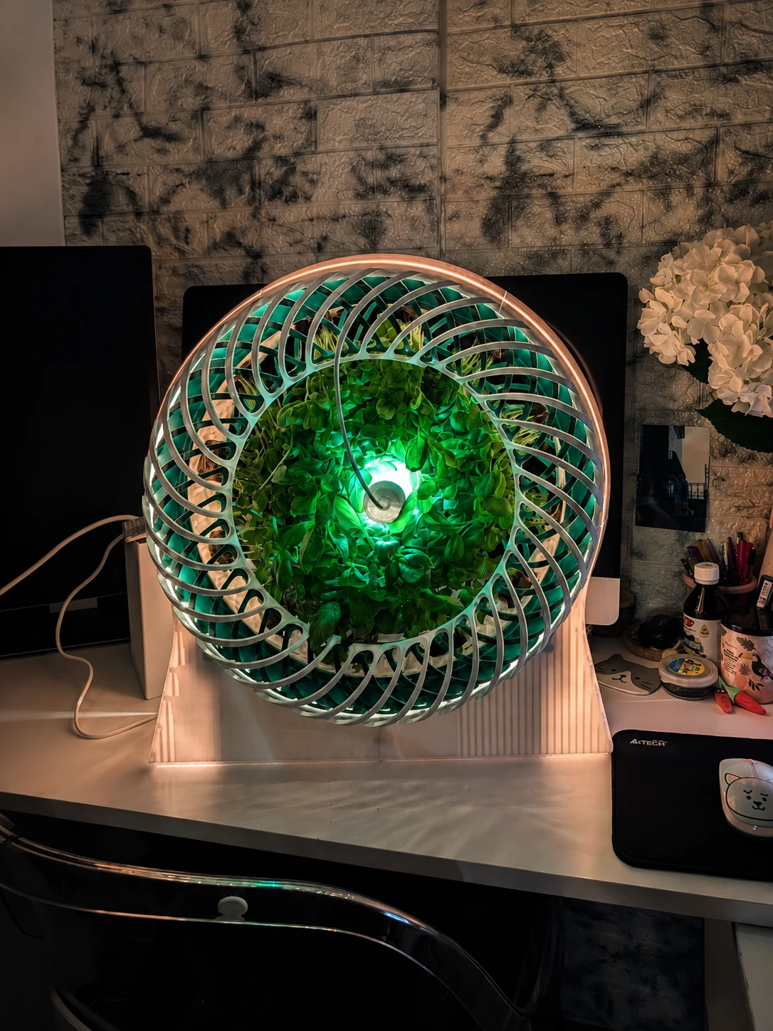
1.1.1What the system controls
FlavoRotor controls the environment delivered to a plant: light, photoperiod, nutrient additions, pH management, electrical conductivity, root-zone temperature, water exposure and rotation. Sensors and actuator logs record what the plant received over time.
From a controlled treatment to a repeatable crop recipe
The machine controls environmental inputs, records the delivered treatment and links it to measured plant responses.
Values
| Series | Value | Note |
|---|---|---|
| Versioned recipe | Setpoints + schedule + limits | A recipe identifies the crop, cultivar, treatment schedule, permitted operating range and the exact recipe version. |
| Calibrated delivery | Light · nutrients · pH · rotation | Actuators translate the recipe into physical inputs. Pump, sensor and light calibration records remain attached to the run. |
| Measured environment | What the plant actually received | Time-series measurements distinguish the commanded setpoint from the environment that was physically delivered. |
| Plant response | Growth · chemistry · aroma · taste | Plant response is measured after treatment. A control command is never treated as a sensory result. |
| Replication | Repeat → compare → version | Replicated runs establish whether a response is associated with the treatment and remains reproducible across cycles. |
FlavoRotor system architecture, represented from internal engineering records I01 and I02.
1.1.2How flavour enters the experiment
Taste, aroma, colour and texture are plant responses. They are measured after a defined cultivation treatment; they are not inferred from a pump command or a single sensor value. Published crop studies show that spectrum, nutrient composition, solution strength and root-zone temperature can change relevant chemical or quality measurements under controlled conditions.
1.1.3What this documentation contains
The following chapters explain the machine, the cultivation variables, crop-specific mechanisms, equations, calibration procedures, experimental designs, chemical analysis, sensory testing and recipe transfer. The complete document is designed to be read continuously from this point.
1.2Research roadmap
1.2.1Objective
FlavoRotor is developed as a programmable cultivation platform. The research objective is to measure how cultivation inputs change plant outcomes, then reproduce the useful responses with the same crop and recorded conditions.
1.2.2Validation stages
| Stage | Question | Release gate |
|---|---|---|
| 1. Engineering calibration | Does each sensor and actuator reproduce its command within a declared uncertainty? | Calibration report and raw data |
| 2. Empty-system mapping | What spatial and temporal gradients exist before plants are added? | Light, temperature, humidity, rotation and reservoir maps |
| 3. Biological baseline | Can one cultivar be grown repeatedly with one fixed recipe? | At least three independent cycles |
| 4. Single-factor screening | Which controllable factor produces a measurable effect? | Preregistered control and treatment comparison |
| 5. Chemical and sensory confirmation | Is the effect chemically measurable and perceptible? | Instrumental analysis plus blinded sensory test |
| 6. Interaction model | How do selected factors interact? | Factorial or response-surface experiment |
| 7. Recipe replication | Can the result be reproduced on another cycle or unit? | Replication report |
| 8. Transfer | Can the recipe be translated to a larger system using physical variables? | Scale-transfer report |
1.2.3Publication rule
Each released result remains linked to its protocol version, biological material, system identifier, calibration records, raw dataset, processing code and conclusion linked to the tested conditions. This structure follows reusable plant-experiment metadata and FAIR data principles.
1.3Terminology and units
1.3.1Core definitions
| Term | Operational definition |
|---|---|
| Taste | Basic gustatory perception such as sweet, sour, bitter, salty or umami |
| Aroma | Olfactory contribution arising predominantly from volatile compounds |
| Flavour | Combined taste, aroma, texture, trigeminal and contextual perception |
| Texture | Mechanical and structural perception measured instrumentally and/or sensorially |
| Recipe | Versioned schedule of measurable cultivation setpoints and actions |
| Biological replicate | An independently grown plant or experimental unit |
| Technical replicate | Repeated measurement of the same biological sample |
| Independent cycle | A cultivation run started at a separate time with a new biological batch |
1.3.2Required units
| Quantity | Symbol | Unit |
|---|---|---|
| Hydrogen-ion activity | pH | dimensionless logarithmic activity scale |
| Electrical conductivity | EC | mS/cm, temperature reported |
| Photon flux density | PPFD | µmol·m⁻²·s⁻¹ |
| Daily light integral | DLI | mol·m⁻²·d⁻¹ |
| Temperature | T | °C |
| Relative humidity | RH | % |
| Vapour-pressure deficit | VPD | kPa |
| Angular speed | n | rev/min |
| Angular velocity | ω | rad/s |
| Flow | Q | mL/min |
| Concentration | c | mmol/L or mg/L, species stated |
| Fresh/dry mass | m | g |
1.3.3Reporting rules
- EC is always reported with solution temperature or temperature compensation.
- pH is reported with calibration date, buffers and electrode identifier.
- Light is reported at plant position, not inferred only from electrical wattage.
- Concentration values identify the chemical species and basis, for example mg/L K rather than “potassium EC”.
- Mean values include variability, sample size and the experimental unit.
1.3.4Metrology source
Accuracy, precision, repeatability, resolution, calibration and uncertainty are used according to international metrology vocabulary and guidance.
2Experimental platform
How the rotating chamber, magnetic transmission, nutrient reservoir, lighting, sensors, imaging, data acquisition and service architecture work together.
2.1Experimental platform
2.1.1Platform purpose
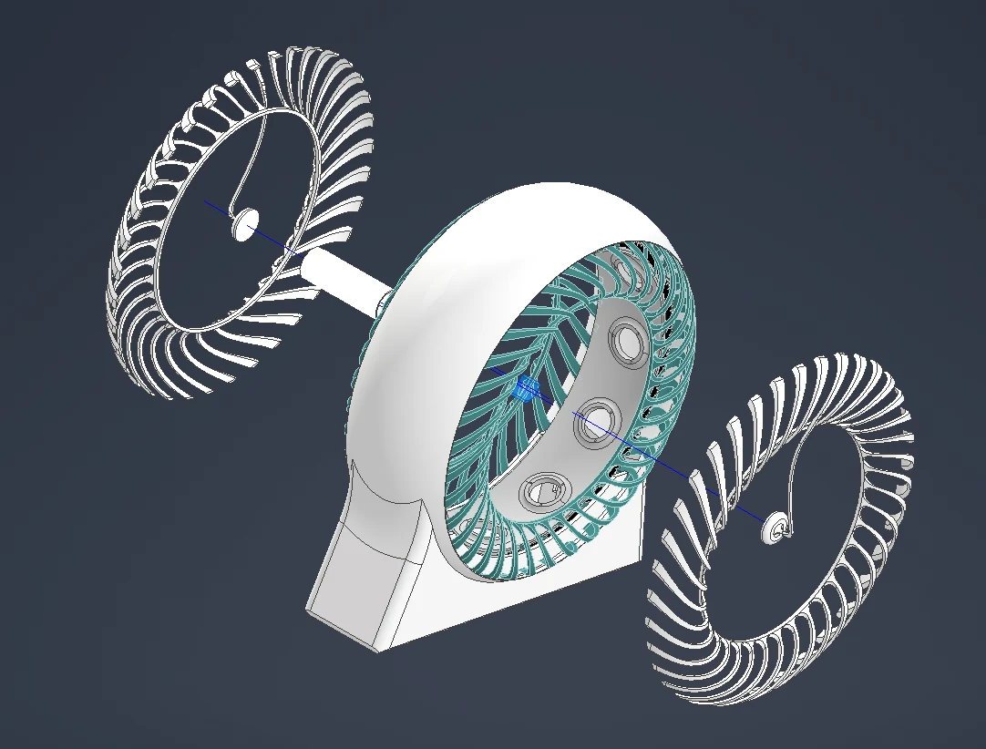
The platform is designed to expose multiple plants to a common, logged environment while allowing programmable changes in cultivation inputs. Its role is not to assume a flavour outcome; its role is to deliver and record treatments with sufficient repeatability to test one.
2.1.2Subsystems
| Subsystem | Controlled or observed quantity | Required validation |
|---|---|---|
| Rotating drum | speed, direction, duty cycle, immersion sequence | RPM trace, position repeatability, vibration, load test |
| Magnetic drive | transmission ratio and overload slip | static slip torque and loaded endurance |
| Axial lighting | spectrum, PPFD, photoperiod | spectroradiometric map and DLI |
| Nutrient reservoir | volume, level, temperature, pH, EC | mixing time, drift, leak and sanitation test |
| Four-channel dosing | stock-liquid volume | channel-specific gravimetric calibration |
| Imaging | repeatable plant image | fixed geometry, exposure and colour reference |
| Data system | timestamped observations and commands | clock, schema, missing-data and audit-log tests |
2.1.3Cultivation cycle
2.1.4Internal engineering records
The supplied v1 project report documents printed mechanical parts, sensor electronics, PCB fabrication, software monitoring and an incompletely assembled final device due to delayed components. The v2 report documents a revised magnetic-drive and four-pump design. This site therefore reports the platform as a documented engineering development; hardware performance is promoted only when a dedicated calibration report exists.
2.1.5FlavoRotor design provenance
The system-specific configuration on this page is traced to the supplied FlavoRotor engineering records.
2.2Version 1.0 to 2.0
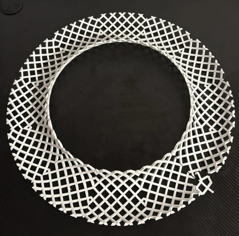
2.2.1Subsystem evolution
| Subsystem | v1 record | v2 record | Research significance |
|---|---|---|---|
| Drive | conventional stepper/roller architecture | magnetic coupling concept | requires new torque and speed calibration |
| Nutrient delivery | manual/general solution control | four custom peristaltic channels | enables versioned experimental dosing after calibration |
| Imaging | monitoring concept | central camera/CNN concept | requires repeatable capture and device-specific dataset |
| Lighting | axial LED concept | specified blue/red/far-red/white concept | requires measured spectrum and spatial map |
| Exterior | functional prototype frame | stationary and rotating design layers | may affect airflow and optical distribution |
| Software | dashboard and taste-profile prototype | recipe/feedback concept | must separate measured variables from sensory outcomes |
2.2.2Research lesson
Every mechanical redesign can change the experimental environment. A recipe validated on v1 cannot be assumed valid on v2 unless light, root-zone exposure, air flow and control performance are shown equivalent.
2.2.3FlavoRotor design provenance
The system-specific configuration on this page is traced to the supplied FlavoRotor engineering records.
2.3Rotating cultivation drum
2.3.1Explanation
Plants are arranged around a cylindrical drum. As the drum turns, each root module passes through the nutrient reservoir and then drains in air. A central light source is intended to keep the plant positions at similar radial distance from the source.
2.3.2Functions to validate
| Function | Engineering metric | Biological risk if uncontrolled |
|---|---|---|
| Rotation | mean RPM, within-cycle variation, direction | unequal immersion and mechanical stimulus |
| Immersion | time in solution, depth, interval | unequal water and nutrient exposure |
| Drainage | retained volume and drain time | root-zone oxygen differences |
| Position balance | radial mass distribution | vibration and speed modulation |
| Plant retention | module force and displacement | plant damage or loss |
| Cleanability | accessible wetted surfaces | biofilm and cross-cycle contamination |
2.3.3Immersion timing
ExplanationOne minute contains 60 seconds, so dividing 60 by the rotation speed gives the time needed for one complete turn.
ExplanationThe fraction of the circle occupied by the nutrient bath is multiplied by the duration of one turn to estimate how long roots remain immersed.
The immersion time must be calculated from the measured contact angle and verified with video or position sensing. It must not be inferred from RPM alone.
2.3.4Biological comparison requirement
A rotation trial needs a static or movement-matched control with equivalent mean DLI, root-zone exposure and air flow. Otherwise light, watering and mechanical effects remain confounded.
2.3.5FlavoRotor design provenance
The system-specific configuration on this page is traced to the supplied FlavoRotor engineering records.
2.4Magnetic drive system
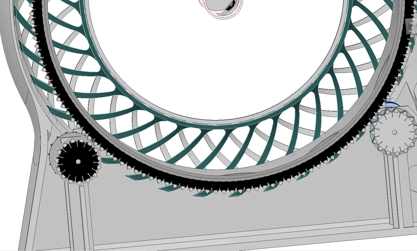
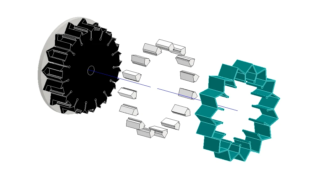

2.4.1Design definition
| Parameter | Design record |
|---|---|
| Driving wheel teeth | 15 |
| Driven wheel teeth | 146 |
| Nominal ratio | 146/15 = 9.733:1 |
| Magnet type | NdFeB N42, Ø8 × 3 mm in the v2 specification |
| Nominal air gap | 2.5 mm in the v2 specification |
| Intended behaviour | non-contact torque transfer with overload slip |
2.4.2Kinematic model
ExplanationThe ratio between driven and driving teeth defines how much the drive reduces speed and increases available torque.
ExplanationDriven speed is motor speed divided by the transmission ratio.
ExplanationDividing 60 by the driven speed gives the duration of one output rotation.
2.4.3Why the earlier force estimate is not a final result
A magnetic dipole approximation can support preliminary sizing, but the short separation, finite cylindrical magnets, alternating polarities, tooth geometry and simultaneous interactions violate the simplest far-field assumptions. The resulting torque must therefore be treated as an analytical estimate, not a verified 3.9 N·m capability.
2.4.4Required validation
| Test | Method | Reported output |
|---|---|---|
| Static slip torque | force gauge at known radius | torque-angle curve and peak slip torque |
| Starting load | incremental drum load | minimum starting torque and motor current |
| Speed stability | encoder or video tachometry | mean RPM, SD and periodic ripple |
| Endurance | loaded operation over defined hours | slip events, temperature and drift |
| Misalignment | controlled axial/radial offset | torque margin and failure threshold |
ExplanationMeasured slip torque is compared with the largest required torque. A value above one leaves a positive operating margin.
2.4.5FlavoRotor design provenance
The system-specific configuration on this page is traced to the supplied FlavoRotor engineering records.
2.5Nutrient reservoir and root-zone exposure
2.5.1Function
The reservoir is both the nutrient-solution storage volume and the sequential root-contact zone. This reduces the need for a separate recirculation circuit, but it makes liquid level, mixing, temperature, oxygen and carry-over central experimental variables.
2.5.2Required reservoir state
| Variable | Why it matters | Minimum record |
|---|---|---|
| Working volume | converts dose volume into concentration change | pre- and post-dose volume or level |
| Liquid level | sets immersion depth and time | continuous or per-cycle level |
| Temperature | affects roots, electrode response and oxygen solubility | logged °C |
| pH | affects nutrient speciation and uptake | calibrated pH trace |
| EC | bulk ionic-strength proxy | temperature-corrected EC trace |
| Dissolved oxygen | root-zone aeration indicator | DO where instrumentation is available |
| Mixing time | determines when feedback is valid | step-response test |
| Sanitation state | controls biological carry-over | cleaning batch and verification |
2.5.3Mixing validation
Inject a harmless conductivity tracer or a small controlled nutrient-stock dose at the normal dosing point. Measure EC at the control sensor and at representative reservoir positions until all readings remain within the predefined mixing tolerance. The maximum observed stabilisation time becomes the minimum feedback delay.
2.5.4Volume balance
ExplanationThe next reservoir volume equals the current volume plus additions, minus sampling and other losses.
2.5.5FlavoRotor design provenance
The system-specific configuration on this page is traced to the supplied FlavoRotor engineering records.
2.6Light, spectrum and DLI
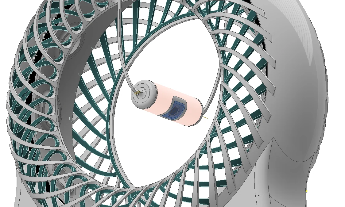
2.6.1Required metrics
| Metric | Definition |
|---|---|
| Spectrum | photon distribution by wavelength at plant position |
| PPFD | instantaneous 400–700 nm photon flux density |
| DLI | daily integrated photosynthetic photon exposure |
| Photoperiod | scheduled light duration |
| Uniformity | spatial distribution across plant positions |
| Leaf temperature | thermal outcome at the tissue, not only room temperature |
ExplanationDaily light is the time integral of photon flux at plant position. For constant PPFD, this reduces to PPFD multiplied by photoperiod in seconds, divided by one million.
2.6.2Published basil study
In hydroponic Italian Large Leaf basil, controlled supplemental-light spectra altered key aroma volatiles under a defined experimental environment. The transferable conclusion is that spectrum is a valid treatment variable. The exact result requires matching cultivar, DLI and other conditions.
2.6.3Why wattage is insufficient
A 50 W electrical rating and manufacturer efficacy estimate cannot define PPFD inside a cylindrical system. Optical distribution, distance, angle, reflection, obstruction, thermal state and plant position must be measured.
2.7Environmental sensing and calibration
2.7.1Measurement principle
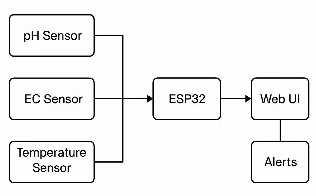
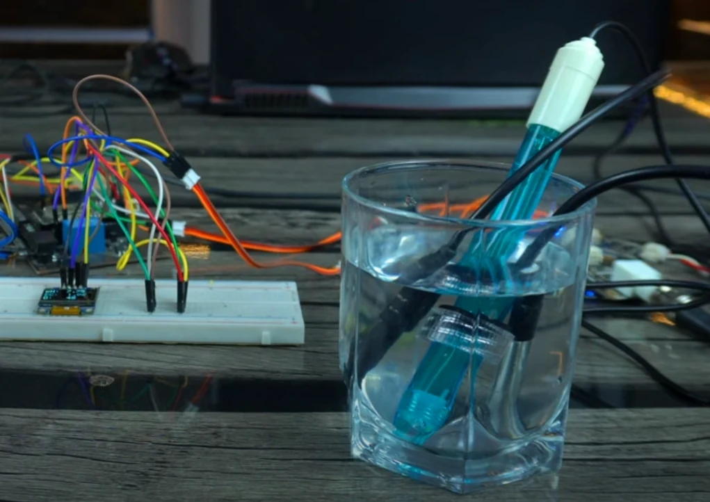
A sensor reading becomes research data only when its identity, calibration, range, sampling interval, temperature conditions and failure rules are recorded.
2.7.2Minimum calibration plan
| Sensor | Calibration/verification | Frequency trigger |
|---|---|---|
| pH | two- or three-point buffers bracketing operation; slope and offset retained | before a trial, after cleaning, on drift or according to electrode stability |
| EC | certified conductivity standard near operating range; temperature compensation checked | before a trial and after probe maintenance |
| Solution temperature | comparison with traceable reference in stirred bath | before deployment and on replacement |
| Level | measured-volume additions across working range | after geometry or sensor position changes |
| PPFD | reference quantum sensor/spectroradiometer mapping | after light, optics or geometry changes |
| Rotation | encoder or video reference across commanded speeds | after drive or load changes |
2.7.3pH electrode model
ExplanationThe ideal electrode voltage changes linearly with pH. Real sensors still require measured slope and offset calibration.
2.7.4Calibration record
calibration_id, sensor_id, sensor_model, serial_number,
reference_standard, reference_lot, reference_value,
measured_value, solution_temperature, fitted_slope,
fitted_offset, residual, operator, timestamp, firmware_version
2.7.5Fault rules
Out-of-range, non-finite, implausibly fast-changing or stale measurements disable automatic correction. The system logs the rejected value and the reason; it does not silently replace it with a plausible number.
2.7.6Traceability
Calibration records identify reference material, method, environmental conditions, corrections and uncertainty.
2.8Data acquisition architecture
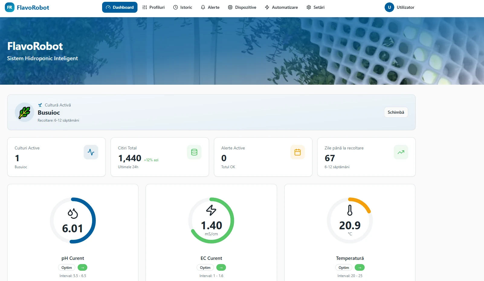
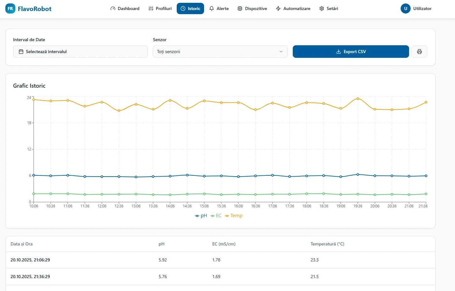
2.8.1Reconstruction requirement
An independent analyst must be able to reconstruct what the system was commanded to do, what it actually measured, what deviations occurred and which samples were harvested.
2.8.2Core data streams
Every published result remains traceable to the cultivation run
Identifiers connect hardware state, sensor streams, recipe versions, images, samples and derived analyses.
Values
| Series | Value | Note |
|---|---|---|
| Cultivation run | run_id | The run record binds system version, crop identity, cultivar, recipe version and start/end timestamps. |
| Raw observations | sensor_id · event_id · image_id | Raw sensor packets, actuator events and images retain timestamps and device identifiers before analysis. |
| Biological samples | plant_id · sample_id | Harvested material remains linked to plant position, cultivation cycle and analytical method. |
| Derived analysis | analysis_id · software_version | Every transformed value records the code or method version and the source observations used to calculate it. |
| Published record | table · figure · dataset | A figure or result resolves back to its exact source table, file and treatment definition. |
FlavoRotor data architecture; MIAPPE and FAIR concepts are described in sources R23 and R24.
| Stream | Examples | Primary key |
|---|---|---|
| System state | mode, faults, firmware, system version | timestamp + system_id |
| Sensors | pH, EC, temperature, level, PPFD reference | timestamp + sensor_id |
| Actuators | pump steps, channel, rotation command, light state | event_id |
| Recipe | time-indexed setpoints and limits | recipe_id + version |
| Biological material | species, cultivar, seed lot, position | sample_id |
| Observations | mass, image, colour, chemistry, sensory | observation_id |
| Calibration | model coefficients and validity | calibration_id |
2.8.3Time integrity
The controller and server clocks are synchronised before a trial. Records use UTC internally and retain the local timezone for human-readable reports. Missing intervals are represented explicitly; time series are never filled silently.
2.8.4Metadata standard
The study package follows MIAPPE concepts for investigation, study, biological material, environment and observed variables, and FAIR principles for durable identifiers and machine-readable metadata.
2.8.5FlavoRotor design provenance
The system-specific configuration on this page is traced to the supplied FlavoRotor engineering records.
2.9Camera, plant phenotyping and machine learning
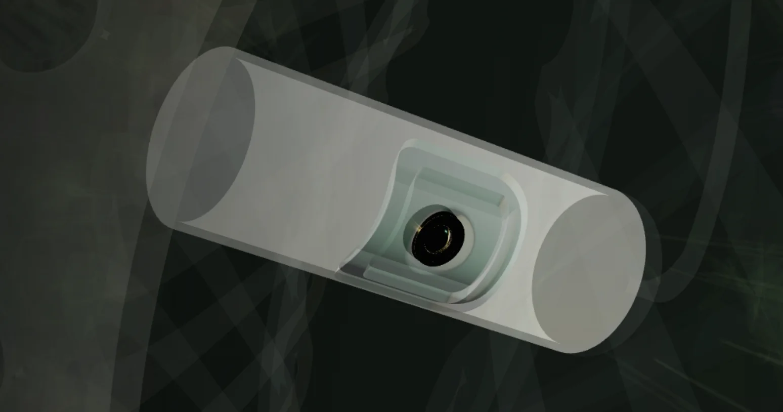
2.9.1Camera geometry
The camera is fixed to the central module. The rotor stops at a known encoder position and presents one plant module to the lens. At that position, the optical axis meets the local plant plane at 90°. The distance, lens and framing therefore remain comparable when the same plant returns for its next image. The acquisition record stores camera version, lens, focus, working distance, encoder position and image dimensions.
Indexed camera geometry
The camera faces the plant module at 90° when the rotor reaches its recorded capture position.
Values
| Series | Value | Note |
|---|---|---|
| Fixed camera | Lens, focus and pose are recorded | The camera remains fixed to the stationary central module. Its lens, focus, working distance and orientation belong to the acquisition record. |
| Optical axis | 90° to the plant plane | At the indexed position, the perpendicular view limits perspective change between observations of the same plant. |
| Indexed rotor position | Position ID and encoder state | A capture is accepted only when the plant module reaches its defined angular position and motion is below the blur threshold. |
| Optical references | Scale, colour and light state | A scale reference and periodic colour target detect changes in camera geometry, illumination and colour rendering. |
Note. FlavoRotor camera geometry is documented in I02. Repeatable phenotyping practice follows Arend et al. (2016).
2.9.2What is stored with each image
The image file alone is not enough. Its record identifies the plant, growth cycle, rotor position, exposure, gain, white balance and light state. A scale reference makes pixel measurements comparable. A colour target reveals changes in illumination or camera response. Focus, clipping and occlusion are stored as visible image-quality fields.
| Field group | Stored values | Reason |
|---|---|---|
| Plant | plant_id, crop, cultivar, seed lot, cycle_id | keeps repeated images attached to one biological specimen |
| Position | position_id, encoder index, camera pose, working distance | shows where and how the image was taken |
| Camera | camera_version, lens, focus, exposure, gain, white balance | separates plant change from camera change |
| Growing conditions | recipe_version, light state, temperature, pH, EC, rotation state | connects the image to the measured environment |
| File history | timestamp_utc, SHA-256, annotation version, operator | identifies the exact file and label version |
2.9.3Images used for model development
Three image sources have different jobs. ImageNet supplies the general visual weights used to initialise MobileNetV2. PlantVillage supplies clean, labelled leaf images. PlantDoc adds leaves photographed with natural backgrounds and changing viewpoints. FlavoRotor images represent the camera, lighting and plant geometry in which the model operates. Results from these sources remain separate because a clean single-leaf photograph is different from a plant growing inside the machine.
| Images | Content | Use |
|---|---|---|
| ImageNet-1K | general photographs from many object classes | initial weights for edges, textures and shapes |
| PlantVillage | 54,306 controlled RGB leaf images covering healthy tissue and plant diseases | controlled leaf-classification benchmark |
| PlantDoc | 2,598 plant images from 13 species and 27 healthy or disease classes | comparison under natural backgrounds and variable framing |
| FlavoRotor | indexed images from the central camera | device-specific plant tracking and evaluation |
The reproducible web example downloads the complete PlantVillage Strawberry RGB subset at repository commit 7f7ecc7: 456 healthy images and 1,109 leaf-scorch images. The repository's published leaf map identifies 1,232 of those images as observations of 190 physical leaves. The Python script records every selected filename, SHA-256 hash, class, leaf group and transform parameter.
PlantVillage strawberry images used in the reproducible example
These are unaltered RGB files from separate published leaf groups. Select an image to inspect its source filename and leaf identifier.
Values
| Series | Value | Note |
|---|---|---|
| Healthy · leaf 49 | Published RGB image · 256 × 256 px | 64aea8c6-24df-40c1-9d68-0221f4151383___RS_HL 2103.JPG · SHA-256 c83901b7…2b5d. |
| Healthy · leaf 57 | Published RGB image · 256 × 256 px | d50fa8fa-015b-41f6-a2aa-18efcf041f6e___RS_HL 2188.JPG · SHA-256 1a40422c…69c4. |
| Healthy · leaf 75 | Published RGB image · 256 × 256 px | 78debbd4-43b4-437d-8fd8-86910b947d34___RS_HL 4459.JPG · SHA-256 3904614b…ac6f. |
| Healthy · leaf 61 | Published RGB image · 256 × 256 px | 411e3372-e40e-44ed-aa47-972afabd15f7___RS_HL 2225.JPG · SHA-256 07c17d2f…24f. |
| Leaf scorch · leaf 69 | Published RGB image · 256 × 256 px | 212433a4-4bda-450e-8026-02ffa42f9f32___RS_L.Scorch 1551.JPG · SHA-256 7c4e91ed…ce81. |
| Leaf scorch · leaf 16 | Published RGB image · 256 × 256 px | 16311953-0608-43c1-829d-d78b990a0fa4___RS_L.Scorch 0995.JPG · SHA-256 5d5f1729…7c55. |
| Leaf scorch · leaf 74 | Published RGB image · 256 × 256 px | f8c43823-8efa-4f97-8e37-8ab7e0115fd0___RS_L.Scorch 1604.JPG · SHA-256 18ac7e23…8e6f. |
| Leaf scorch · leaf 60 | Published RGB image · 256 × 256 px | d0d0377c-6c41-4bb4-abd8-f21553d37c09___RS_L.Scorch 1459.JPG · SHA-256 041c90ad…26a. |
Note. Images from the PlantVillage Strawberry RGB subset (Mohanty, Hughes, & Salathé, 2016), repository commit 7f7ecc7, CC BY-SA 3.0. Displayed at a common size without synthetic symptoms.
2.9.4Split by physical leaf
Photographs of the same physical leaf stay together. The deterministic seed 20260729 assigns leaf groups to 70% training, 15% validation and 15% test partitions. This prevents near-duplicate photographs of one leaf from appearing in both training and test data.
| Class | Training | Validation | Test |
|---|---|---|---|
| Healthy | 316 images / 80 leaves | 68 images / 17 leaves | 72 images / 18 leaves |
| Leaf scorch | 534 images / 52 leaves | 115 images / 11 leaves | 127 images / 12 leaves |
| Total | 850 images / 132 leaves | 183 images / 28 leaves | 199 images / 30 leaves |
2.9.5Image augmentation
The Python preprocessing script creates the examples below from one published leaf-scorch image. Rotation, scale, brightness, contrast, saturation, blur and sensor noise change the complete frame by a recorded amount. They do not paint new spots or remove existing tissue. Only the training partition receives random augmentation; validation and test images keep their original pixels apart from the fixed resize and normalisation.
Deterministic augmentation examples
The Python script applies small, recorded changes to one published image. It does not draw, remove or recolour a symptom.
Values
| Series | Value | Note |
|---|---|---|
| Original | No transform | Published PlantVillage RGB source image. The repository JPEG remains unchanged. |
| Geometry | Rotation +6° · scale 0.96 · translation 2.5% / 2% | A deterministic affine transform reproduces a small indexing and framing difference. |
| Brightness and colour | Brightness 1.07 · contrast 1.10 · saturation 0.96 | The transform changes the complete frame uniformly; it does not add a local lesion. |
| Blur and sensor noise | Gaussian blur 0.7 px · noise σ = 2/255 | The deterministic example represents a small optical and sensor difference. |
Note. Source image: PlantVillage Strawberry leaf scorch, leaf group 69, commit 7f7ecc7, CC BY-SA 3.0. Parameters and SHA-256 hashes are stored in manifest.json. Transform structure follows Buslaev et al. (2020).
2.9.6MobileNetV2 and the MLP classifier
The reference model receives a 224 × 224 sRGB image. MobileNetV2, initialised with ImageNet-1K weights, converts the image into a 7 × 7 × 1,280 feature map. Global average pooling produces a 1,280-value vector. The MLP maps that vector to 256 ReLU6 units, applies dropout 0.25, and produces one logit for every declared plant-health class.
| Stage | Shape | Operation |
|---|---|---|
| Input | 224 × 224 × 3 | sRGB image with ImageNet normalisation |
| Encoder | 7 × 7 × 1,280 | MobileNetV2 features |
| Pooling | 1,280 | global average pooling |
| Hidden layer | 256 | linear layer, ReLU6 and dropout 0.25 |
| Output | C | one logit per class |
| Probability | C | softmax followed by validation-set temperature scaling |
Why this model fits the camera task
MobileNetV2 uses depthwise convolutions and inverted residual blocks. With the 256-unit classifier, it contains 2,586,434 parameters. The same camera is evaluated at every indexed plant position, so model size and single-image latency matter alongside classification performance.
The classifier head
Global average pooling converts the 7 × 7 × 1,280 encoder output into one 1,280-value feature vector. The multilayer perceptron learns combinations of those features that separate the declared classes. ReLU6 bounds each hidden activation between 0 and 6; dropout removes 25% of hidden activations at random during fitting. The final linear layer returns two logits, which softmax converts into class probabilities.
ExplanationThe frozen image encoder produces a feature vector. A 256-unit hidden layer transforms it, dropout regularises training and the output layer produces one score for each class.
The 1,280 × 256 hidden layer has 327,680 weights and 256 biases. The 256 × 2 output has 512 weights and 2 biases. The MLP therefore contributes 328,450 trainable parameters.
Encoder comparison
MobileNetV2, EfficientNetB0 and ResNet50 were tested with the same frozen ImageNet protocol, 256-unit ReLU6 MLP, physical-leaf split and three deterministic seeds. All three reached 100% mean accuracy on the 199-image controlled test. The natural-background PlantDoc check separated them: mean healthy-class recall was 84.38% for MobileNetV2, 74.65% for EfficientNetB0 and 55.90% for ResNet50.
Image encoder comparison
Same frozen ImageNet encoder protocol, grouped data split, MLP head and three seeds.
Values
| Series | Value | Note |
|---|---|---|
| MobileNetV2 | PlantDoc healthy recall 84.38% · median CPU latency 60.59 ms | 2,586,434 parameters; 10.35 MB FP32 parameter memory; controlled grouped-test accuracy 100.00%; external recall range 81.25–88.54% across three deterministic seeds. |
| EfficientNetB0 | PlantDoc healthy recall 74.65% · median CPU latency 83.35 ms | 4,378,021 parameters; 17.51 MB FP32 parameter memory; controlled grouped-test accuracy 100.00%; external recall range 67.71–81.25% across three deterministic seeds. |
| ResNet50 | PlantDoc healthy recall 55.90% · median CPU latency 171.27 ms | 24,112,770 parameters; 96.45 MB FP32 parameter memory; controlled grouped-test accuracy 100.00%; external recall range 40.63–71.88% across three deterministic seeds. |
PlantVillage controlled test and PlantDoc natural-background transfer check; TensorFlow 2.18 CPU inference on an Intel Xeon E5-2699 v3 with a three-core Docker limit.
MobileNetV2 also required the fewest parameters and had the lowest measured CPU latency: 2.59 million parameters and 60.59 ms median, compared with 4.38 million and 83.35 ms for EfficientNetB0, and 24.11 million and 171.27 ms for ResNet50. Latency was measured with TensorFlow 2.18 inside a three-core Docker limit on an Intel Xeon E5-2699 v3. Processor choice changes throughput, not the mathematical definition of accuracy.
Five-fold grouped cross-validation
A second test used all 1,232 images tied to 190 physical leaves. The folds were stratified by class; every leaf appeared in one test fold and never in that fold’s training or validation data. MobileNetV2 and the MLP were refitted in every fold. Aggregate accuracy was 99.84%, balanced accuracy 99.87% and macro F1 99.83%; two of 776 leaf-scorch images were assigned healthy and all 456 healthy images were assigned correctly. Mean PlantDoc healthy recall across the five fitted models was 80.00% with a standard deviation of 8.38 percentage points.
Five-fold physical-leaf cross-validation
Every one of 190 physical leaves appears in one test fold and never in that fold’s training or validation data.
Values
| Series | Value | Note |
|---|---|---|
| Fold 1 | Controlled accuracy 100.00% · PlantDoc healthy recall 87.50% | 248 test images from 38 physical leaves; confusion matrix [[92, 0], [0, 156]]. |
| Fold 2 | Controlled accuracy 99.61% · PlantDoc healthy recall 73.96% | 255 test images from 38 physical leaves; confusion matrix [[92, 0], [1, 162]]. |
| Fold 3 | Controlled accuracy 99.59% · PlantDoc healthy recall 68.75% | 242 test images from 38 physical leaves; confusion matrix [[90, 0], [1, 151]]. |
| Fold 4 | Controlled accuracy 100.00% · PlantDoc healthy recall 82.29% | 247 test images from 38 physical leaves; confusion matrix [[90, 0], [0, 157]]. |
| Fold 5 | Controlled accuracy 100.00% · PlantDoc healthy recall 87.50% | 240 test images from 38 physical leaves; confusion matrix [[92, 0], [0, 148]]. |
MobileNetV2 with a refitted 256-unit ReLU6 MLP in each fold; 1,232 grouped PlantVillage Strawberry images and a separate 96-image PlantDoc transfer check.
The image classifier assigns one of its declared visual labels to the current frame. Biomass forecasting, nutrient-state estimation and stress attribution use separate models with repeated images and measured cultivation variables.
Image capture, model and review
Each result remains attached to the image, plant, cultivation cycle, camera settings and model version.
Values
| Series | Value | Note |
|---|---|---|
| Indexed RGB capture | Image and acquisition record | The image is stored with plant, cycle, position, recipe, camera, exposure and illumination identifiers. |
| Image check | Focus, exposure, occlusion and pose | Images outside declared quality limits are rejected before segmentation or classification. |
| Feature encoder | MobileNetV2 · 224 × 224 px | The convolutional encoder provides an efficient feature representation. ImageNet pretraining supplies generic visual features, not plant-health labels. |
| MLP classifier | 1,280 → 256 → C | Global-average-pooled features pass through a 256-unit ReLU6 layer, dropout 0.25 and a final C-class linear layer. |
| Confidence | Temperature-scaled probabilities | One scalar temperature is fitted on the validation set so reported confidence better matches observed correctness. |
| Plant history | Repeated observations of one plant | A persistent change across indexed captures carries more evidential weight than an isolated frame. |
Note. The encoder follows MobileNetV2 (Sandler et al., 2018), initialised with ImageNet weights (Deng et al., 2009); confidence calibration follows Guo et al. (2017).
2.9.7Model fitting
- Fit the MLP.The ImageNet encoder remains frozen while the classifier learns from the grouped training images.
- Fine-tune the final encoder blocks.A lower learning rate adjusts the highest-level visual features; validation macro F1 controls early stopping.
- Calibrate probability.One temperature value is fitted to validation logits after the model weights stop changing.
- Lock the test.Architecture, preprocessing, class thresholds and the low-confidence rule are fixed before test images are opened.
- Report each image domain separately.PlantVillage, PlantDoc and FlavoRotor results use separate tables, because their camera conditions differ.
Training and validation accuracy by epoch
The encoder was frozen for three epochs, then its final blocks were fine-tuned for two epochs. Select an epoch to inspect the recorded accuracy and loss.
Accuracy · vertical scale 0.9500–1.0000
Values
| Series | Value | Note |
|---|---|---|
| Epoch 1 · classifier head | Training accuracy 0.9918 · validation accuracy 1.0000 | Training loss 0.021185 · validation loss 0.000098. |
| Epoch 2 · classifier head | Training accuracy 1.0000 · validation accuracy 1.0000 | Training loss 0.000333 · validation loss 0.000033. |
| Epoch 3 · classifier head | Training accuracy 1.0000 · validation accuracy 1.0000 | Training loss 0.000354 · validation loss 0.000014. |
| Epoch 4 · fine-tuning | Training accuracy 0.9765 · validation accuracy 1.0000 | Training loss 0.072895 · validation loss 0.000014. |
| Epoch 5 · fine-tuning | Training accuracy 0.9847 · validation accuracy 1.0000 | Training loss 0.055849 · validation loss 0.000015. |
Note. TensorFlow 2.18.0 run completed 29 July 2026 with seed 20260729. Values are read directly from training-history.csv; the vertical axis is limited to 0.95–1.00 so small changes remain visible.
2.9.8Controlled-image benchmark
The reproducible TensorFlow 2.18.0 run completed on 29 July 2026. After five epochs, the locked model classified all 199 images in the grouped PlantVillage test partition correctly: 72 healthy and 127 leaf scorch. The test partition contains 30 physical leaf groups that were absent from training and validation. Accuracy, macro F1 and balanced accuracy are each 1.0000 for this controlled two-class benchmark. The fitted temperature is 0.500584 and the ten-bin expected calibration error is 0.0000361.
Controlled Strawberry test-set classifications
Rows are published PlantVillage labels and columns are model predictions. Select a cell to inspect the exact count.
Predicted class
199 images · 30 physical leaf groups · 199 correct classifications
Values
| Series | Value | Note |
|---|---|---|
| Actual healthy · predicted healthy | 72 images | All 72 healthy test images were assigned to the healthy class. |
| Actual healthy · predicted leaf scorch | 0 images | No healthy test image was assigned to leaf scorch. |
| Actual leaf scorch · predicted healthy | 0 images | No leaf-scorch test image was assigned to healthy. |
| Actual leaf scorch · predicted leaf scorch | 127 images | All 127 leaf-scorch test images were assigned to leaf scorch. |
Note. The leaf-grouped test partition contains 199 previously withheld images from 30 physical leaves. The complete TensorFlow run and model hash are recorded in training-summary.json.
PlantVillage photographs isolated leaves against a controlled background. The result above therefore measures discrimination between those two published Strawberry classes under the same acquisition style; it is not substituted for a measurement from the FlavoRotor camera.
Uncertainty around the measured scores
Every classification score is estimated from a finite test set. The controlled test observed 199 correct assignments from 199 images, but its exact two-sided 95% interval is 98.16–100%. Class recall has wider intervals because each class contains fewer observations: 95.01–100% for 72 healthy images and 97.14–100% for 127 leaf-scorch images. The interval states how much precision the test count provides; it does not change the observed confusion matrix.
Performance estimates with exact 95% confidence intervals
A perfect observed score from a finite controlled test still has uncertainty. The natural-background check is lower and wider.
Values
| Series | Value | Note |
|---|---|---|
| Controlled test accuracy | 100.00% · 95% CI 98.16–100.00% | 199 correct outcomes from 199 published test observations. The interval is the two-sided 95% Clopper–Pearson exact binomial interval. |
| Controlled healthy recall | 100.00% · 95% CI 95.01–100.00% | 72 correct outcomes from 72 published test observations. The interval is the two-sided 95% Clopper–Pearson exact binomial interval. |
| Controlled leaf-scorch recall | 100.00% · 95% CI 97.14–100.00% | 127 correct outcomes from 127 published test observations. The interval is the two-sided 95% Clopper–Pearson exact binomial interval. |
| PlantDoc healthy-class recall | 82.29% · 95% CI 73.17–89.33% | 79 of 96 healthy-labelled natural-background images were assigned healthy. Brier score 0.1662; mean confidence among the 17 wrong assignments 94.26%. |
Note. Two-sided Clopper–Pearson intervals calculated from the locked test counts. PlantVillage and PlantDoc are reported separately because their image domains differ.
2.9.9Natural-background check
The frozen model was then applied without retraining to all 96 images in PlantDoc's Strawberry leaf class. These photographs contain natural backgrounds, changing scale, partial leaves and varied lighting. The model assigned 79 images to healthy and 17 to leaf scorch, which gives healthy-class recall of 79 / 96 = 0.8229. PlantDoc does not publish a matching Strawberry leaf-scorch class, so this check reports recall for its healthy class rather than two-class accuracy.
Natural-background Strawberry images from PlantDoc
The same frozen model was applied to PlantDoc images labelled Strawberry leaf. Three low-confidence-order and three high-confidence-order examples are shown.
Values
| Series | Value | Note |
|---|---|---|
| PlantDoc image 1 | Upstream label: healthy · predicted leaf scorch | Fragaria-virginiana-6.jpg · P(healthy) 0.000000025 · SHA-256 49738f34…93b1. |
| PlantDoc image 2 | Upstream label: healthy · predicted leaf scorch | 102_0829.JPG.jpg · P(healthy) 0.000008215 · SHA-256 1e5a93bc…6097. |
| PlantDoc image 3 | Upstream label: healthy · predicted leaf scorch | img_0164.jpg · P(healthy) 0.000009111 · SHA-256 47344a43…69a3. |
| PlantDoc image 4 | Upstream label: healthy · predicted healthy | indian-strawberry-leaf.jpg · P(healthy) > 0.999999999999 · SHA-256 0d2b7902…d94e. |
| PlantDoc image 5 | Upstream label: healthy · predicted healthy | Strawberry+leaves.jpg · P(healthy) > 0.999999999999 · SHA-256 368f4a9c…af54. |
| PlantDoc image 6 | Upstream label: healthy · predicted healthy | strawberry-plant-leaves-strawberry-red-spots-on-strawberry-plant-leaves.jpg · P(healthy) 1.000000 · SHA-256 5cb64d2e…728c. |
Note. Images from the PlantDoc Strawberry leaf class (Singh et al., 2020), repository commit 5467f60, CC BY 4.0. Labels shown here are the upstream dataset labels; probabilities are produced by the recorded FlavoRotor reference run.
2.9.10Metric definitions
Precision answers: of the images assigned to one class, how many are correct? Recall answers: of the images that truly belong to that class, how many were found? F1 combines both values. Macro F1 gives every class the same weight, so the larger leaf-scorch class cannot hide weak performance on healthy leaves. The report also contains the complete confusion matrix, balanced accuracy, image count and physical-leaf count for every class.
ExplanationF1 combines precision and recall. Macro F1 is the arithmetic mean of the class-level F1 values, so a large class cannot hide poor performance on a smaller class.
ExplanationPredictions are grouped into confidence bins. ECE is the weighted difference between observed accuracy and mean reported confidence in those bins.
2.9.11Following one plant through time
Repeated images of the same plant form a time series. Projected canopy area, calibrated colour, developmental stage and image quality are stored beside temperature, light, pH, EC and recipe version at the same timestamp. Growth rate compares the same plant at two recorded times. It does not compare unrelated plants photographed on different days.
| Output | Reference annotation | Use |
|---|---|---|
| Canopy area and growth rate | manual masks and a physical scale reference | tracks the plant's visible growth |
| Developmental stage | crop-specific, expert-reviewed labels | aligns treatment timing with plant development |
| Colour index | colour target and matching laboratory measurements | measures visible colour change |
| Plant-health class | expert label and supporting laboratory result where required | records class and probability for review |
| Image quality | focus, exposure, occlusion and pose labels | identifies unsuitable images |
Datasets used to test longitudinal methods
| Dataset | Repeated observations | Role in the research programme |
|---|---|---|
| Aalto lettuce | 18 identified heads, 30 biomass days, 731 canopy images and 1,443 environmental records | implemented three-day biomass forecast with plant-wise validation |
| HydroGrowNet | three 30-day Batavia cycles and more than 390,000 segmented images aligned with pH, EC and water temperature | independent multimodal growth and anomaly dataset |
| Multi-sensor lettuce phenotyping | 45 plants over 42 days, two cultivars, three nitrogen levels and two irrigation rates | external RGB, 3D, multispectral, SPAD, fluorescence and morphology dataset |
A separate model for each measured endpoint
| Question | Model | Reason | Reference value |
|---|---|---|---|
| Does the current leaf image match a declared visual class? | MobileNetV2 + 256-unit MLP | compact image encoder; class probabilities can be calibrated and reviewed | expert or published class label |
| What fresh biomass is expected three days from now? | ridge autoregression | uses repeated mass and recent growth increments while regularising a small dataset | measured fresh biomass |
| How did cultivar and nutrient solution change tissue chemistry? | factorial ANOVA | tests cultivar, treatment and their interaction directly | laboratory nitrogen, sulphate, organic acid and chlorophyll measurements |
| Is the plant departing from its expected trajectory? | forecast residual plus consecutive-capture rule | requires persistence through time and retains the sensor and image context | next measured observation |
2.9.12Stored model output
Every model output stores the image hash, plant ID, model version, preprocessing version, probability for every class, calibrated confidence and image-quality score. A low-quality or low-confidence image is marked for review together with the reason. The original image and complete class-probability vector remain available beside the final label.
2.10Perimeter status lighting
2.10.1Purpose
The perimeter lighting communicates operating state, warnings, service conditions and user interactions without changing the central cultivation-light recipe. Colour assignments are interface states and are versioned in the software configuration.
| Function | Required behaviour | Research relevance |
|---|---|---|
| Normal operation | stable, low-glare indication | must not alter a declared dark period |
| Warning | visible, distinct state | event is written to the operating record |
| Critical fault | unambiguous alert | associated actuator state and timestamp are preserved |
| Service mode | local identification of the active module | prevents maintenance events from being hidden in a trial |
2.10.2Engineering requirements
- exact LED family and revision recorded in the bill of materials;
- maximum and typical channel current measured on the installed assembly;
- voltage drop measured at the first, middle and final segment;
- surface and enclosure temperature recorded at worst-case command;
- power-supply headroom, connector rating and conductor cross-section documented;
- brightness limited for night operation and camera acquisition;
- status meanings remain accessible through text or the dashboard and do not rely on colour alone.
2.10.3Validation plan
Bench validation records current, voltage, temperature and command latency for representative patterns. Optical validation records spectrum and PPFD at plant positions with the central lamp off and on. Trial protocols state whether perimeter lighting was disabled, constant or included in the measured recipe.
2.10.4Permitted claims
The website may state that the v2.0 architecture includes addressable perimeter status lighting. It may not state that the subsystem supplements photosynthesis, improves flowering or delivers a defined wavelength until a component-specific spectrum and plant-position photon map are published.
2.11Industrial design and serviceability
2.11.1Scope
Industrial design is included in the research documentation because enclosure decisions can alter access, airflow, light distribution, camera visibility, contamination risk and mechanical balance. Aesthetic intent is recorded separately from measured cultivation performance.
2.11.2Layered architecture
The v2.0 concept separates a stationary external frame from the rotating cultivation layer. This allows plant movement to remain visible while fixed guards, service panels, lighting and cable routes remain referenced to the structure. The original prototype and v2.0 reports provide the primary engineering record.
2.11.3Serviceability requirements
| Area | Requirement | Verification output |
|---|---|---|
| Plant modules | individual removal without disturbing unrelated samples | tool list, access sequence and measured service time |
| Nutrient reservoir | inspection, draining and cleaning without wetting electronics | drain test and cleaning record |
| Pump tubing | replacement with channel identity preserved | replacement procedure and post-service calibration check |
| Lighting and camera | fixed optical reference after service | position check and image/light revalidation |
| Rotating assembly | guard clearance under maximum declared load | clearance and interference inspection |
| Materials | compatibility with moisture, nutrient solution and cleaning method | material record and inspection interval |
2.11.4Verification plan
Verification includes assembly and disassembly trials, loaded rotation, splash observation, cable-clearance inspection, access-time measurement, cleaning inspection and confirmation that service work does not invalidate sensor, pump, camera or light calibration. Deviations are recorded as maintenance events in the experiment log.
3Nutrient dosing
How the custom peristaltic pump, calibration procedure, four dosing channels, stock solutions, control logic and fluidic safeguards work.
3.1Peristaltic pump development
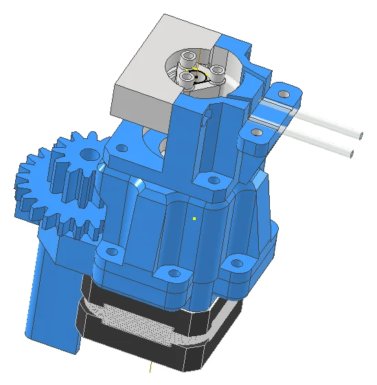
3.1.1Explanation
A three-roller rotor compresses a flexible tube. Advancing the compression moves liquid while the liquid remains inside the replaceable tube. The motor provides a precise command, but only calibration determines the volume that actually exits the tube.
3.1.2Documented design
| Parameter | v2 design value | Classification |
|---|---|---|
| Pump type | three-roller peristaltic | design architecture |
| Tube | 3.2 mm ID / 6.4 mm OD silicone | design specification |
| Nominal channel radius | 18 mm | CAD specification |
| Drive | NEMA 17, 1.8° full step, direct drive | component specification |
| Command mode | 1/16 microstepping | firmware design |
| Housing | PETG prototype geometry | CAD specification |
| System channels | four independent pump modules | system design |
3.1.3First-order model
ExplanationTube area is calculated from its internal diameter.
ExplanationIdeal volume per turn is tube area multiplied by the effective squeezed length and the number of displacement events.
With di = 3.2 mm, Leff = 25 mm and Ne = 3, the report model gives At ≈ 8.04 mm² and Vrev,ideal ≈ 0.603 mL/rev.
ExplanationThe ideal volume is corrected by an efficiency measured on the real pump.
ExplanationFlow equals delivered volume per turn multiplied by turns per minute.
3.1.4Motor-command increment
ExplanationMotor step angle and microstepping determine how many commands produce one rotor revolution.
ExplanationNominal volume per command is the measured volume per revolution divided by commands per revolution.
3.1.5Why calibration is mandatory
Tube recovery, occlusion, viscosity, suction head, outlet pressure, roller geometry, motor torque, microstep non-linearity and tube wear all alter delivered volume. Peristaltic-pump modelling and published multi-channel systems therefore use physical calibration rather than geometry alone.
3.1.6Progress classification
The pump geometry and four-channel module are substantial v2 engineering progress. The supplied report documents CAD, component selection and the analytical model. No traceable FlavoRotor gravimetric dataset accompanies the report, so delivered-volume performance remains unclaimed until CR-PMP-001 is published.
3.1.7FlavoRotor design provenance
The system-specific configuration on this page is traced to the supplied FlavoRotor engineering records.
3.1.8CAD documentation
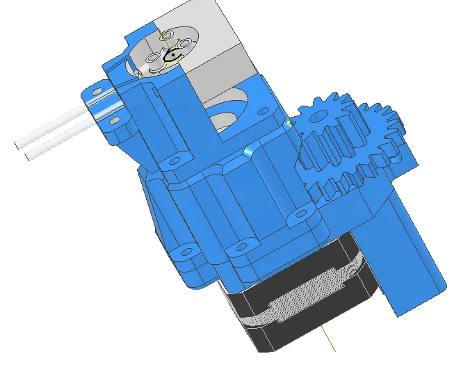
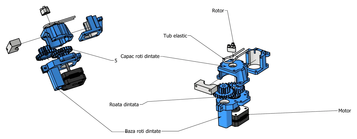
3.2Gravimetric pump calibration
3.2.1Principle
Each pump dispenses into a vessel on a calibrated balance. Mass gain is converted to volume using fluid density at the measured temperature. The test is repeated across channel, dose, speed, tube condition and hydraulic head.
ExplanationThe mass gained by the receiving vessel is converted into liquid volume using density at the measured temperature.
ExplanationMean flow is delivered volume divided by run time.
The gravimetric chain follows traceable liquid-volume and uncertainty principles: balance performance, test-liquid density, evaporation, timing, repeatability and calibration state are recorded. Large published peristaltic-pump datasets show why repeated measurements and drift analysis are necessary, but their performance values are not transferred to FlavoRotor.
3.2.2Test matrix
| Factor | Levels |
|---|---|
| Channel | 1, 2, 3, 4 |
| Rotor speed | 5, 15, 30 and 60 rev/min |
| Commanded dose | 0.5, 1, 2, 5 and 10 mL |
| Repetitions | minimum 20 per primary condition |
| Fluid | deionised water and each representative stock class |
| Tube state | new, mid-life and replacement threshold |
| Hydraulic condition | minimum, nominal and maximum inlet head; installed outlet path |
| Direction | forward; reverse purge characterised separately |
3.2.3Calibration statistics
ExplanationThe arithmetic mean combines all repeated delivery measurements.
ExplanationBias is the difference between the mean delivered volume and the requested volume.
ExplanationThe coefficient of variation expresses repeatability spread as a percentage of the mean.
ExplanationRMSE combines all deviations from the requested volume into one error value.
Repeatability, bias, residual analysis and method precision are reported using declared statistical procedures rather than a single R² value.
3.2.4Channel model
ExplanationThe first calibration model links command count to delivered volume; residuals show whether a more complex model is needed.
3.2.5Predefined engineering acceptance gates
| Metric | Gate for initial reservoir dosing |
|---|---|
| Relative bias | ≤ ±3% for doses ≥1 mL within the declared range |
| Repeatability | CV ≤2% for doses ≥1 mL |
| Channel model | residual structure absent and R² reported, not used alone |
| Drift | ≤5% before recalibration or tube replacement |
| Cross-channel contamination | none detected above method limit |
| Backflow/siphon | no uncontrolled transfer in the installed hydraulic range |
These are FlavoRotor acceptance criteria, not claimed achieved performance. Published multi-channel pump data guide the method but are not copied as FlavoRotor results.
3.2.6FlavoRotor design provenance
The system-specific configuration on this page is traced to the supplied FlavoRotor engineering records.
3.3Four-channel nutrient dosing module
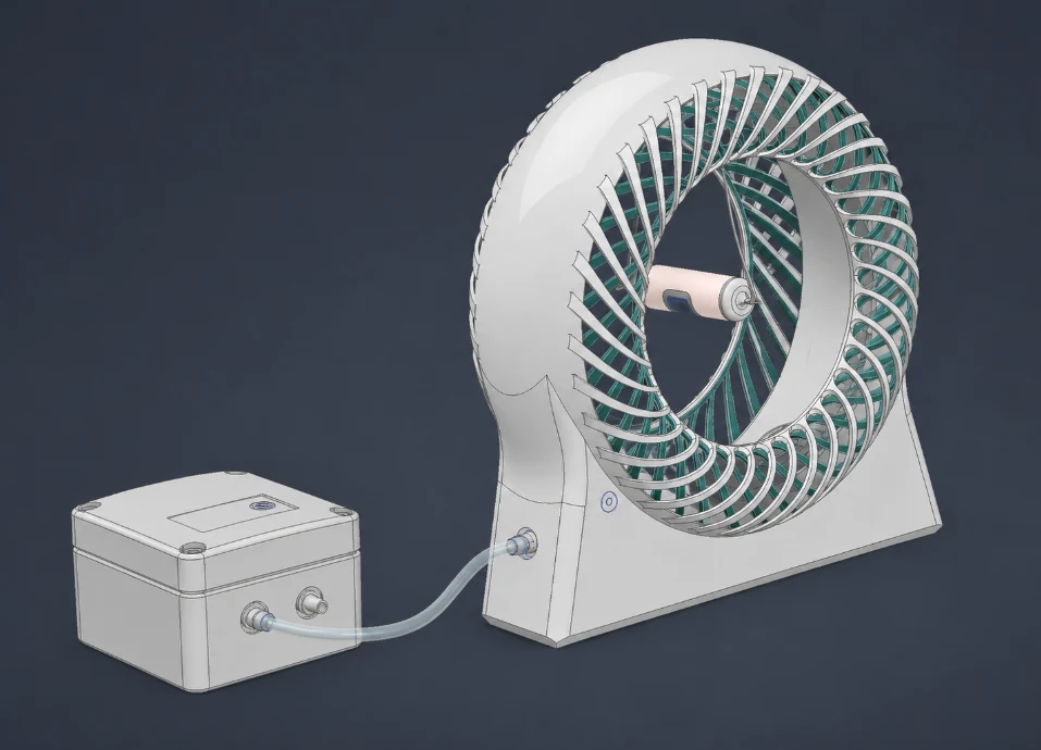
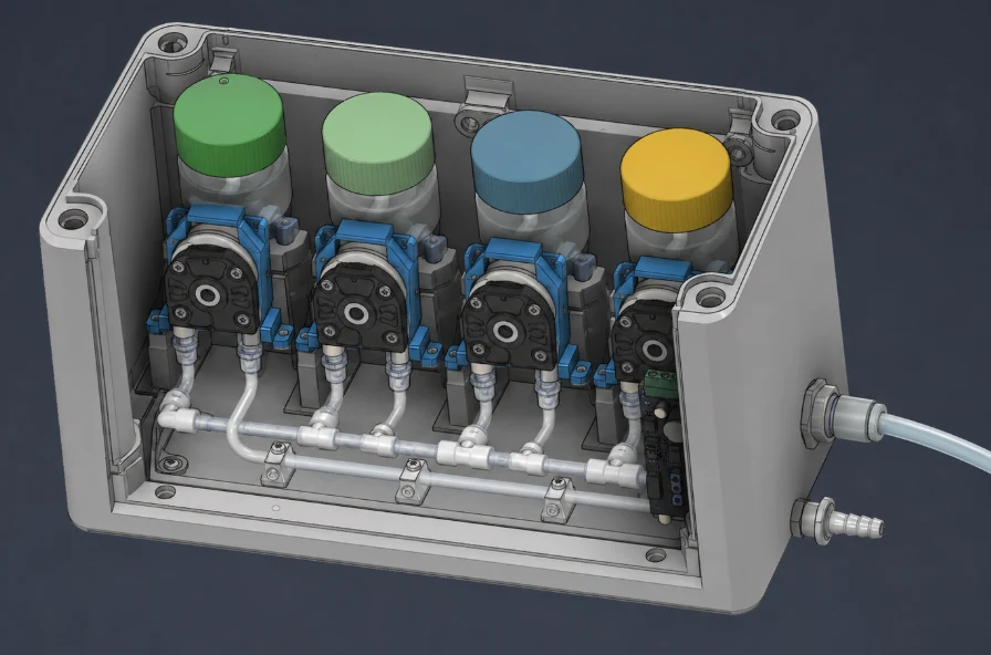
3.3.1Explanation
Four pumps allow four liquids to be added independently. The channels control liquid volumes. They do not directly control sweetness, acidity or aroma.
3.3.2Architecture
The documented motor-control architecture uses STEP/DIR microstepping drivers of the A4988 class. Driver selection defines command generation and protection requirements; it does not determine pump volumetric accuracy.
3.3.3Safe channel definition
| Channel | Permitted role | Required metadata |
|---|---|---|
| 1 | water or defined stock | fluid ID, batch and density |
| 2 | nutrient stock A | full chemical composition and compatibility class |
| 3 | nutrient stock B | full chemical composition and compatibility class |
| 4 | correction or experimental stock | purpose, maximum dose and exclusion rules |
3.3.4Dose traceability
event_id, timestamp, system_id, recipe_id, recipe_version,
channel_id, fluid_id, fluid_batch, calibration_id,
requested_volume_mL, commanded_steps, speed_rpm, direction,
reservoir_volume_before_L, pH_before, EC_before, temperature_before,
mixing_delay_s, pH_after, EC_after, fault_state
3.3.5FlavoRotor design provenance
The system-specific configuration on this page is traced to the supplied FlavoRotor engineering records.
3.3.6Module interior
3.4Nutrient stock solutions
3.4.1Principle
Each stock solution is defined by the concentration of every relevant chemical species, not by a marketing label. The controller calculates the amount added to the reservoir from calibrated dose volume and stock composition.
ExplanationThe concentration increase depends on stock strength and dose volume, then is diluted by the reservoir volume.
ExplanationThe next ion inventory includes new additions and subtracts plant uptake and losses.
3.4.2Stock compatibility
Concentrated calcium stocks are separated from concentrated phosphate or sulphate stocks unless compatibility has been demonstrated, because precipitation can remove nutrients and obstruct tubing. Stock identity, concentration, solvent, preparation date, lot and storage conditions are recorded.
3.4.3Recipe solving
When several stocks contribute to several ions, the system solves a constrained non-negative dosing problem rather than assigning one pump to one sensory attribute.
ExplanationThe controller converts each candidate stock volume into a reservoir concentration change, then selects non-negative volumes that approach the target without exceeding dose limits.
3.4.4Ion coupling
Stock design accounts for the fact that fertilizer salts introduce coupled ions and that precise individual-ion control requires more information than bulk EC.
3.5Nutrient dosing control strategy
3.5.1Control hierarchy
3.5.2Variables suitable for direct feedback
- reservoir level or working volume;
- bulk EC, with temperature compensation;
- pH, with calibrated electrode and mixing delay;
- solution temperature;
- dissolved oxygen if a validated sensor is installed.
Sweetness, acidity of harvested tissue and aroma are not direct loop variables because they are not measured continuously in the reservoir.
3.5.3Discrete PI form
ExplanationControl error is simply the target value minus the measured value.
ExplanationThe controller reacts to the present error and to accumulated error over time.
ExplanationThe requested action is kept between declared minimum and maximum limits.
3.5.4Dose sequence
- Validate sensor state and reservoir volume.
- Calculate a bounded stock-volume request.
- Verify channel calibration and stock identity.
- Deliver dose and log actuator command.
- Wait the measured mixing time.
- Acquire stable pH/EC readings.
- Apply another correction only if all limits remain valid.
3.5.5pH control note
Because pH is logarithmic and buffering varies with solution composition, the controller uses small empirical dose increments and measured response rather than converting pH error directly into a fixed acid/base volume. Open-source pH-stat work supports this calibration and logging approach.
3.6Fluidic safety and maintenance
3.6.1Mandatory interlocks
| Condition | Automatic response |
|---|---|
| Invalid or stale sensor | block feedback correction |
| Reservoir below minimum level | block concentrated stock dosing |
| Reservoir above maximum level | block water addition |
| Calibration expired | block volumetric automatic dosing |
| Maximum dose/runtime exceeded | stop channel and latch fault |
| Mixing delay active | block second feedback action |
| Stock mismatch | reject recipe execution |
| Cover/service state unsafe | disable pump motion where required |
| Communication loss | outputs return to defined safe state |
| Leak detected | stop all liquid actuators and alert |
3.6.2Tube lifecycle
Tube service life is not published as a fixed 1,000-hour value unless validated for the exact tube, occlusion, fluid, speed and duty cycle. Replacement is triggered by calibrated-flow drift, visible damage, loss of occlusion, contamination risk or the validated service threshold.
3.6.3Cleaning record
cleaning_id, system_id, channel_id, cleaning_agent,
concentration, contact_time, rinse_volume, verification_method,
operator, timestamp, next_allowed_fluid_class
3.6.4FlavoRotor design provenance
The system-specific configuration on this page is traced to the supplied FlavoRotor engineering records.
4Flavour control
How measured cultivation conditions can influence plant chemistry, aroma, taste, colour and texture, from pH and nutrients to light, root conditions and harvest.
4.1What flavour means
4.1.1Explanation
Flavour is not one sensor value. It is the combined experience produced by taste, retronasal aroma, texture, temperature, trigeminal sensations and context.
4.1.2FlavoRotor outcome model
| Outcome | Example measurements | What it cannot prove alone |
|---|---|---|
| Taste | sweet, sour, bitter, salty, umami intensity | volatile aroma composition |
| Aroma | descriptor profile, GC–MS volatile abundance | consumer preference |
| Texture | firmness, fracture, fibrousness, juiciness | taste identity |
| Appearance | instrumental colour, morphology, visible defects | flavour quality |
| Difference | triangle or other discrimination test | direction or preference |
| Liking | consumer hedonic score | chemical cause |
Discrimination, descriptive profiling and consumer liking answer different questions and are documented separately.
4.1.3Core rule
4.1.4Measurement map
| Term | What is measured | Suitable method |
|---|---|---|
| Taste | sweet, sour, bitter, salty and umami sensations | trained descriptive panel or defined consumer method |
| Aroma | orthonasal and retronasal odour attributes | descriptive sensory analysis; VOC analysis as complementary evidence |
| Flavour | integrated taste, aroma and trigeminal perception | sensory method selected for the claim |
| Texture | firmness, crispness, fibrousness and juiciness | instrumental texture plus sensory description |
| Preference | degree of liking | consumer hedonic test; never inferred from chemistry alone |
Terminology and method selection follow sensory-analysis standards. A chemical difference can help explain perception, but it does not replace a sensory test.
4.1.5A measurable sensory fingerprint
A target is stored as a versioned set of measurements for one crop and cultivar at a defined harvest stage. It combines a small number of primary chemical and sensory variables with physical plant state and the complete cultivation history.
| Layer | Examples of recorded variables | Method |
|---|---|---|
| Chemistry | selected volatile compounds, sugars, organic acids, pigments | validated chromatographic or spectrometric method |
| Sensory | sweet, sour, bitter, named aromas, texture, trigeminal sensations | coded and blinded sensory protocol |
| Physical state | developmental stage, colour, fresh and dry mass, water content | calibrated imaging and physical measurements |
| Process history | light, temperature, humidity, nutrient, pH, EC, rotation and harvest history | timestamped sensor and actuator records |
4.2How cultivation steers flavour
4.2.1Definition of control
FlavoRotor defines a reproducible flavour result when a requested target can be translated into a versioned cultivation recipe that produces a statistically and sensorially bounded outcome across independent cycles.
4.2.2Controllable inputs
The platform can programme light, nutrient-stock additions, pH management, bulk EC limits, solution temperature and rotation schedule; the supplied engineering reports also document the rotating drum, sensing, monitoring and proposed four-channel dosing architecture.
4.2.3Measured outcomes
Outcomes are crop-specific: basil may be evaluated through selected aroma volatiles and descriptive aroma; arugula through glucosinolate-related phytochemicals, pungency and bitterness; lettuce through bitterness, texture and quality; mint through essential-oil composition and menthol-related descriptors; strawberry through soluble solids, titratable acidity, volatile profile, firmness and sensory response.
4.2.4Recipe model
ExplanationA plant-quality result is modelled from cultivation conditions, genetics, system state and growth stage, plus unexplained variation.
The model is trained only after single-factor and interaction experiments. It is never seeded with invented nutrient-to-flavour coefficients.
4.2.5Recipe release gate
A recipe is released only when the machine input was calibrated, the protocol was frozen before analysis, the result includes uncertainty and effect size, sensory evidence is appropriate to the claim, and at least one independent replication succeeds.
4.2.6From influence to repeatable targeting
- Measure influence.Change one calibrated input and measure the chemical and sensory response against a matched control.
- Map the response.Repeat across treatment levels and independent cycles to estimate direction, magnitude and interaction with cultivar and growth stage.
- Define a target.Freeze the chemical, sensory and physical acceptance ranges before a new cultivation run begins.
- Test prospectively.Run the frozen recipe on new biological material and compare the harvest with the predefined target.
- Replicate.Repeat on another cycle, unit and operator with the same physical targets and calibrated local commands.
4.3pH management
4.3.1Explanation
pH changes the chemical environment around the roots. It affects nutrient speciation, solubility, microbial conditions and uptake. It is not a direct “sweetness dial”.
ExplanationpH is a logarithmic expression of active hydrogen ions; one pH unit represents a tenfold change.
4.3.2Published crop studies
Lettuce studies show that relatively small pH changes can alter physiological performance and tissue composition. These studies justify a pH trial but do not demonstrate a universal taste setting.
4.3.3Operational approach
| Step | Requirement |
|---|---|
| Select setpoint | crop, cultivar, formulation and literature anchor stated |
| Calibrate | buffers bracket expected operating range |
| Measure | temperature and stabilisation criteria recorded |
| Correct | small bounded acid/base increments |
| Mix | wait validated mixing time |
| Re-read | require stable repeated measurements |
| Publish | report actual pH distribution, not only nominal target |
4.3.4How to test pH and flavour correctly
Use at least three pH treatments while keeping elemental formulation, EC, DLI, temperature, harvest age and post-harvest handling matched. Measure tissue composition, biomass, chemistry and blinded sensory response. A difference in growth alone is not a flavour result.
4.4EC and ionic balance
4.4.1Explanation
EC measures how well the solution conducts electricity. It is useful for detecting overall dilution or concentration, but it cannot state how much potassium, nitrate, calcium or magnesium is present individually.
ExplanationMeasured conductivity is corrected to 25 °C so readings taken at different temperatures can be compared.
4.4.2Ion drift
Plant uptake is selective. A controller can hold bulk EC near target while individual ions diverge. This is directly documented in hydroponic nutrient-dynamics research.
4.4.3Required controls
- known initial elemental composition;
- logged stock additions and water additions;
- reservoir-volume accounting;
- periodic solution replacement or laboratory verification;
- crop-specific tissue or solution analysis for research claims;
- EC used as a bulk constraint, not an ion sensor.
4.4.4EC experiment rule
An EC treatment is reproducible only when the recipe used to reach that EC is also specified. Raising EC with a balanced nutrient concentrate is biologically different from raising EC with NaCl or a single salt, even when the meter reads the same value.
4.5Nutrient composition, plant chemistry and stock design
4.5.1Explanation
Adding one fertilizer changes every ion carried by that salt. A KNO₃ dose changes both potassium and nitrate; it is not a pure “sweetness” command.
4.5.2Mass balance
ExplanationThe new amount of one ion equals the previous amount plus stock additions, minus plant uptake and losses.
ExplanationFinal concentration is the final ion amount divided by the final mixed solution volume.
4.5.3Separate N, P and K limitation
The USDA Bibb lettuce dataset changes one target nutrient concentration at a time and reports fresh mass through day 32 after transplant. The day-32 response is not monotonic for every nutrient. Nitrogen rises from 1.16 g at 5 mg·L⁻¹ to 250.73 g at 132 mg·L⁻¹, then falls to 74.11 g at 264 mg·L⁻¹. Phosphorus rises from 9.14 g at 1 mg·L⁻¹ to 250.73 g at 31 mg·L⁻¹. The potassium series contains a wide interval at 42 mg·L⁻¹, so that treatment mean should not be read without its uncertainty.
Fresh mass under separate nitrogen, phosphorus and potassium limitation
Each panel preserves the nutrient's own concentration scale. Points show the authors’ day-32 treatment mean and published 95% interval.
Values
| Series | Value | Note |
|---|---|---|
| Nitrogen · 5 mg·L⁻¹ | 1.16 ± 0.37 g | Treatment mean fresh mass at day 32 after transplant; ± is the published 95% confidence-interval half-width. |
| Nitrogen · 11 mg·L⁻¹ | 32.57 ± 9.22 g | Treatment mean fresh mass at day 32 after transplant; ± is the published 95% confidence-interval half-width. |
| Nitrogen · 26 mg·L⁻¹ | 56.62 ± 21.95 g | Treatment mean fresh mass at day 32 after transplant; ± is the published 95% confidence-interval half-width. |
| Nitrogen · 33 mg·L⁻¹ | 47.73 ± 7.35 g | Treatment mean fresh mass at day 32 after transplant; ± is the published 95% confidence-interval half-width. |
| Nitrogen · 66 mg·L⁻¹ | 100.42 ± 24.14 g | Treatment mean fresh mass at day 32 after transplant; ± is the published 95% confidence-interval half-width. |
| Nitrogen · 132 mg·L⁻¹ | 250.73 ± 25.41 g | Treatment mean fresh mass at day 32 after transplant; ± is the published 95% confidence-interval half-width. |
| Nitrogen · 264 mg·L⁻¹ | 74.11 ± 10.90 g | Treatment mean fresh mass at day 32 after transplant; ± is the published 95% confidence-interval half-width. |
| Phosphorus · 1 mg·L⁻¹ | 9.14 ± 4.57 g | Treatment mean fresh mass at day 32 after transplant; ± is the published 95% confidence-interval half-width. |
| Phosphorus · 2 mg·L⁻¹ | 59.23 ± 14.68 g | Treatment mean fresh mass at day 32 after transplant; ± is the published 95% confidence-interval half-width. |
| Phosphorus · 5 mg·L⁻¹ | 133.56 ± 18.20 g | Treatment mean fresh mass at day 32 after transplant; ± is the published 95% confidence-interval half-width. |
| Phosphorus · 12 mg·L⁻¹ | 176.31 ± 21.98 g | Treatment mean fresh mass at day 32 after transplant; ± is the published 95% confidence-interval half-width. |
| Phosphorus · 31 mg·L⁻¹ | 250.73 ± 25.41 g | Treatment mean fresh mass at day 32 after transplant; ± is the published 95% confidence-interval half-width. |
| Potassium · 2 mg·L⁻¹ | 22.76 ± 4.89 g | Treatment mean fresh mass at day 32 after transplant; ± is the published 95% confidence-interval half-width. |
| Potassium · 13 mg·L⁻¹ | 61.17 ± 6.97 g | Treatment mean fresh mass at day 32 after transplant; ± is the published 95% confidence-interval half-width. |
| Potassium · 21 mg·L⁻¹ | 84.91 ± 16.06 g | Treatment mean fresh mass at day 32 after transplant; ± is the published 95% confidence-interval half-width. |
| Potassium · 42 mg·L⁻¹ | 128.31 ± 174.63 g | Treatment mean fresh mass at day 32 after transplant; ± is the published 95% confidence-interval half-width. |
| Potassium · 105 mg·L⁻¹ | 89.75 ± 30.96 g | Treatment mean fresh mass at day 32 after transplant; ± is the published 95% confidence-interval half-width. |
| Potassium · 210 mg·L⁻¹ | 128.71 ± 15.45 g | Treatment mean fresh mass at day 32 after transplant; ± is the published 95% confidence-interval half-width. |
Note. Values reproduced from Sharkey, Chen, and Altman (2025), author-formatted NPK.CrossT.All.xlsx, day 32 after transplant. No curve was fitted and no point was interpolated.
The graph preserves each nutrient's actual concentration scale and the authors' 95% confidence intervals. It demonstrates two practical points: nutrient response can be curved rather than linear, and equal EC values do not imply equal elemental availability.
4.5.4Nutrient solution and tissue chemistry
El-Nakhel and colleagues tested green and red lettuce with calcium-, magnesium- or potassium-dominant macrocation ratios. The complete design contains three biological replicates in each of six cultivar-by-solution cells. The published measurements include total nitrogen, sulphate, six organic acids and total chlorophyll.
Nutrient-solution composition altered measured lettuce chemistry
Rows combine cultivar and dominant macrocation. Colour is normalised only within each chemical measurement; select a cell for the original unit.
Values
| Series | Value | Note |
|---|---|---|
| Green lettuce · Calcium solution · N | 42.729 g·kg⁻¹ DW | Mean of n = 3 biological replicates; SD 0.506 g·kg⁻¹ DW; SE 0.292 g·kg⁻¹ DW. |
| Green lettuce · Calcium solution · Sulphate | 1.061 g·kg⁻¹ DW | Mean of n = 3 biological replicates; SD 0.014 g·kg⁻¹ DW; SE 0.008 g·kg⁻¹ DW. |
| Green lettuce · Calcium solution · Malate | 41.351 g·kg⁻¹ DW | Mean of n = 3 biological replicates; SD 2.188 g·kg⁻¹ DW; SE 1.263 g·kg⁻¹ DW. |
| Green lettuce · Calcium solution · Chlorophyll | 130.271 mg·kg⁻¹ FW | Mean of n = 3 biological replicates; SD 13.968 mg·kg⁻¹ FW; SE 8.065 mg·kg⁻¹ FW. |
| Green lettuce · Magnesium solution · N | 38.760 g·kg⁻¹ DW | Mean of n = 3 biological replicates; SD 0.421 g·kg⁻¹ DW; SE 0.243 g·kg⁻¹ DW. |
| Green lettuce · Magnesium solution · Sulphate | 1.073 g·kg⁻¹ DW | Mean of n = 3 biological replicates; SD 0.113 g·kg⁻¹ DW; SE 0.066 g·kg⁻¹ DW. |
| Green lettuce · Magnesium solution · Malate | 34.167 g·kg⁻¹ DW | Mean of n = 3 biological replicates; SD 0.832 g·kg⁻¹ DW; SE 0.481 g·kg⁻¹ DW. |
| Green lettuce · Magnesium solution · Chlorophyll | 145.958 mg·kg⁻¹ FW | Mean of n = 3 biological replicates; SD 4.858 mg·kg⁻¹ FW; SE 2.805 mg·kg⁻¹ FW. |
| Green lettuce · Potassium solution · N | 45.565 g·kg⁻¹ DW | Mean of n = 3 biological replicates; SD 0.155 g·kg⁻¹ DW; SE 0.089 g·kg⁻¹ DW. |
| Green lettuce · Potassium solution · Sulphate | 1.578 g·kg⁻¹ DW | Mean of n = 3 biological replicates; SD 0.125 g·kg⁻¹ DW; SE 0.072 g·kg⁻¹ DW. |
| Green lettuce · Potassium solution · Malate | 50.179 g·kg⁻¹ DW | Mean of n = 3 biological replicates; SD 1.064 g·kg⁻¹ DW; SE 0.614 g·kg⁻¹ DW. |
| Green lettuce · Potassium solution · Chlorophyll | 146.668 mg·kg⁻¹ FW | Mean of n = 3 biological replicates; SD 8.080 mg·kg⁻¹ FW; SE 4.665 mg·kg⁻¹ FW. |
| Red lettuce · Calcium solution · N | 42.696 g·kg⁻¹ DW | Mean of n = 3 biological replicates; SD 0.613 g·kg⁻¹ DW; SE 0.354 g·kg⁻¹ DW. |
| Red lettuce · Calcium solution · Sulphate | 1.813 g·kg⁻¹ DW | Mean of n = 3 biological replicates; SD 0.011 g·kg⁻¹ DW; SE 0.006 g·kg⁻¹ DW. |
| Red lettuce · Calcium solution · Malate | 35.763 g·kg⁻¹ DW | Mean of n = 3 biological replicates; SD 1.308 g·kg⁻¹ DW; SE 0.755 g·kg⁻¹ DW. |
| Red lettuce · Calcium solution · Chlorophyll | 275.600 mg·kg⁻¹ FW | Mean of n = 3 biological replicates; SD 6.060 mg·kg⁻¹ FW; SE 3.499 mg·kg⁻¹ FW. |
| Red lettuce · Magnesium solution · N | 45.620 g·kg⁻¹ DW | Mean of n = 3 biological replicates; SD 0.498 g·kg⁻¹ DW; SE 0.287 g·kg⁻¹ DW. |
| Red lettuce · Magnesium solution · Sulphate | 1.589 g·kg⁻¹ DW | Mean of n = 3 biological replicates; SD 0.055 g·kg⁻¹ DW; SE 0.032 g·kg⁻¹ DW. |
| Red lettuce · Magnesium solution · Malate | 42.815 g·kg⁻¹ DW | Mean of n = 3 biological replicates; SD 2.346 g·kg⁻¹ DW; SE 1.354 g·kg⁻¹ DW. |
| Red lettuce · Magnesium solution · Chlorophyll | 288.813 mg·kg⁻¹ FW | Mean of n = 3 biological replicates; SD 1.735 mg·kg⁻¹ FW; SE 1.002 mg·kg⁻¹ FW. |
| Red lettuce · Potassium solution · N | 46.449 g·kg⁻¹ DW | Mean of n = 3 biological replicates; SD 0.472 g·kg⁻¹ DW; SE 0.273 g·kg⁻¹ DW. |
| Red lettuce · Potassium solution · Sulphate | 2.258 g·kg⁻¹ DW | Mean of n = 3 biological replicates; SD 0.178 g·kg⁻¹ DW; SE 0.103 g·kg⁻¹ DW. |
| Red lettuce · Potassium solution · Malate | 55.918 g·kg⁻¹ DW | Mean of n = 3 biological replicates; SD 3.158 g·kg⁻¹ DW; SE 1.823 g·kg⁻¹ DW. |
| Red lettuce · Potassium solution · Chlorophyll | 233.377 mg·kg⁻¹ FW | Mean of n = 3 biological replicates; SD 8.128 mg·kg⁻¹ FW; SE 4.692 mg·kg⁻¹ FW. |
Note. Means calculated from the complete 2 × 3 × 3 design published by El-Nakhel et al. (2020). The downloadable table includes each replicate, standard deviation, standard error and two-way ANOVA output.
A balanced two-way fixed-effects ANOVA was recomputed from all 18 published observations. For malate, the nutrient-solution effect was F(2, 12) = 106.39 with Holm-adjusted p = 3.94 × 10⁻⁷, and the cultivar-by-solution interaction was F(2, 12) = 21.40 with adjusted p = 9.93 × 10⁻⁴. For total chlorophyll, the interaction was F(2, 12) = 25.38 with adjusted p = 4.89 × 10⁻⁴. The interaction means the solution effect changes with cultivar; one universal nutrient-to-chemistry coefficient would discard that structure.
Estimating plant nutrient state
Visible colour is useful but not chemically specific. Nitrogen limitation, water stress, senescence, exposure error and disease can all alter RGB appearance. FlavoRotor therefore joins four records at the same plant and time: the delivered elemental formulation, pH and EC history, the repeated image, and a reference measurement such as tissue mineral composition or chlorophyll. A supervised model predicts a declared laboratory endpoint, not an undefined label such as “nutrient health”.
ExplanationEstimated plant state combines a recent image sequence, delivered treatments, measured environmental conditions, cultivar and day after transplant.
Evaluation keeps all observations from one plant or cultivation cycle in the same fold. The report includes MAE for continuous chemistry, balanced accuracy for declared deficiency classes, calibration of uncertainty and performance for each cultivar and growth stage.
4.5.5Why EC is insufficient
EC is an indirect bulk response to all dissolved ions. Closed systems can maintain a target EC while individual nutrients become deficient or excessive.
4.5.6Four-channel implication
The four FlavoRotor channels must be assigned to chemically defined and compatible fluids. Channel labels describe the liquid, not an expected flavour. The formulation must account for coupled ions, precipitation risk, source-water composition and the limited degrees of freedom available with four reservoirs.
4.5.7Validation
Recipe trials report the full elemental formulation, source water, pH, EC, solution replacement, delivered stock volumes and tissue composition. Sensory conclusions are made only after chemical and blinded sensory measurements.
4.6Light as a flavour-control variable
4.6.1Light variables
| Variable | Required record |
|---|---|
| Spectrum | measured spectral photon distribution at plant positions |
| PPFD | instantaneous photon flux density and spatial map |
| DLI | integrated daily photons |
| Photoperiod | on/off schedule and transitions |
| Far-red | separate 700–750 nm photon record |
| Timing | developmental stage and pre-harvest treatment duration |
Hydroponic Italian Large Leaf basil provides direct evidence that lighting quality can alter key aroma volatiles.
Far-red photons can contribute to canopy photosynthesis when combined with shorter wavelengths, so FlavoRotor records them rather than reducing the light description to “red/blue percentages”.
4.6.2Experimental design
To test a spectral effect, DLI, temperature, cultivar, nutrient formulation, plant age and harvest handling remain matched. A treatment is reported as measured photon distributions, not LED control percentages.
4.6.3Required treatment definition
A light treatment is fully specified only when spectrum, PPFD, DLI, photoperiod, fixture geometry, plant position, leaf temperature and treatment timing are recorded. Percent dimmer settings are device commands, not transferable biological units.
| Variable | Primary measurement | Potential response |
|---|---|---|
| Spectrum | spectral photon distribution | morphology, volatile and secondary-metabolite profile |
| PPFD | µmol·m⁻²·s⁻¹ at plant positions | instantaneous photon exposure |
| DLI | mol·m⁻²·d⁻¹ | daily integrated exposure |
| Photoperiod | hours per day and schedule | development and circadian response |
| Leaf temperature | contact or calibrated infrared measurement | separates optical and thermal effects |
4.7Root-zone environment
4.7.1Scope
Root-zone behaviour is defined by more than pH and EC. FlavoRotor records solution temperature, dissolved oxygen when available, immersion timing, drainage, mixing time, reservoir volume, solution age and root architecture.
4.7.2Temperature
Root-zone temperature can alter growth and soluble-solids measurements, with cultivar-dependent responses reported in lettuce.
4.7.3Reservoir age and composition
Recycled solution can accumulate unwanted or slowly consumed ions while bulk EC remains near target.
4.7.4Sequential immersion
The rotating geometry introduces periodic root wetting and drainage documented in the FlavoRotor system records. This is treated as an experimental factor and potential confounder rather than assumed to improve oxygenation or flavour.
4.7.5Required measurements
- solution temperature at defined locations and intervals;
- reservoir volume and replacement events;
- mixing-time validation after each dose;
- root-zone exposure duration per revolution;
- root images and root dry mass;
- water and nutrient balance.
4.7.6Coupled variables
Root-zone temperature changes oxygen solubility and root metabolism; pH changes nutrient speciation and availability; EC describes bulk conductivity but not individual ions; flow and immersion determine renewal around the root surface. These variables are therefore logged together and are not interpreted independently when they covary.
| Variable | Control purpose | Failure mode to detect |
|---|---|---|
| Solution temperature | stable root-zone condition | heating, cooling or spatial gradients |
| Dissolved oxygen | root respiration support | low oxygen after warming or biological load |
| pH | defined root-zone chemistry | drift, probe fouling or dosing overshoot |
| EC | bulk concentration guardrail | dilution, concentration or ionic imbalance hidden by total EC |
| Immersion and drainage | repeatable wetting cycle | unequal contact, retained liquid or blocked drainage |
4.8Salinity, water stress and multimodal detection
4.8.1Explanation
A treatment can increase the concentration of a compound per gram while reducing total plant growth. Both outcomes must be reported.
4.8.2Response model
ExplanationConcentration alone can rise when a plant becomes smaller. Multiplying by dry mass reveals the total compound produced per plant.
Mint species show species-dependent essential-oil and antioxidant responses under salinity, accompanied by growth effects.
Arugula EC trials report simultaneous changes in growth, nutritional quality and flavour-related phytochemicals, demonstrating why yield and chemistry must be analysed together.
4.8.3Measured water-stress sequence
Fevgas and colleagues published 145 hourly soil-moisture records with RGB, thermal and pseudo-colour lettuce images. The normally irrigated sequence starts at 75% and ends at 73%. The non-irrigated sequence starts at 75% and ends at 8%. A difference of at least 10 percentage points persists from 14 January 2024 at 09:24:45 (UTC+2).
Water availability and image-derived stress signals change on different scales
The upper panel contains every hourly moisture record. The lower panel measures a fixed colour rule on the authors’ pseudo-colour outputs.
Values
316 observations.
Note. Fevgas et al. (2025), CC BY 4.0. Sensor values and pseudo-colour images are reproduced from the published dataset. The two-plant sequence illustrates measurement alignment and is not used as a population estimate.
The lower panel applies one fixed pixel rule to the authors' pseudo-colour outputs: R > 180, G > 180, B < 130 and R + G > 420. Yellow overlay occupies 35.13–52.28% of the detected canopy in the 13 non-irrigated outputs and 0.02–4.11% in the irrigated outputs. This is a measurement of the published visualisation, not a newly trained disease or stress classifier.
Published pseudo-colour outputs for irrigated and non-irrigated lettuce
The authors’ images are shown at their original aspect ratio. No generated plant image or synthetic stress region is added.
Values
| Series | Value | Note |
|---|---|---|
| Irrigated · capture 1 | Published pseudo-colour output | Source file Normal_1.jpg. Full frame retained; no generated or edited plant content. |
| Irrigated · capture 7 | Published pseudo-colour output | Source file Normal_7.jpg. Full frame retained; no generated or edited plant content. |
| Irrigated · capture 13 | Published pseudo-colour output | Source file Normal_13.jpg. Full frame retained; no generated or edited plant content. |
| Non-irrigated · capture 1 | Published pseudo-colour output | Source file Stressed_1.jpg. Full frame retained; no generated or edited plant content. |
| Non-irrigated · capture 7 | Published pseudo-colour output | Source file Stressed_7.jpg. Full frame retained; no generated or edited plant content. |
| Non-irrigated · capture 13 | Published pseudo-colour output | Source file Stressed_13.jpg. Full frame retained; no generated or edited plant content. |
Note. Hybrid-framework pseudo-colour images from Fevgas et al. (2025), CC BY 4.0. The fixed yellow-pixel calculation is documented in summary.json.
Separating water, nutrient and disease signals
A colour change is not assigned a cause from RGB alone. Water stress is checked against reservoir level, root-zone contact, temperature and moisture or water-potential measurements. Nutrient state is checked against the delivered formulation, pH, EC and tissue analysis. Disease labels require symptom-specific expert or laboratory confirmation. The same image can contribute features to each analysis, but each endpoint has its own reference measurement.
Time to detection
For a new cultivation run, detection time is measured from the recorded treatment change to the first alert that remains above threshold for a declared number of consecutive captures. The report includes false-alert rate in control plants, sensitivity, median detection delay and an interval across biological replicates. This distinguishes early detection from a visually strong endpoint image.
4.8.4FlavoRotor rule
No salinity or water-stress recipe is released without biomass, tissue water, visual quality, chemical endpoints and sensory confirmation. Severe stress is not used merely to create a larger analytical signal.
4.9Harvest and post-harvest control
4.9.1Why this matters
A cultivation treatment can be overwhelmed by differences introduced during harvest, storage or sample preparation. Post-harvest conditions are therefore controlled as part of the experiment rather than treated as logistics.
Lettuce quality and shelf-life responses depend on nutrient treatment, season and post-harvest handling.
4.9.2Required harvest record
| Field | Requirement |
|---|---|
| Developmental age | days after sowing and transplanting |
| Time of harvest | clock time and light-cycle position |
| Sample location | defined leaf, fruit or canopy position |
| Pre-analysis delay | minutes or hours |
| Storage | temperature, humidity, package and duration |
| Preparation | washing, cutting, mass and serving temperature |
4.9.3Sensory samples
Samples receive blind random codes, balanced serving order and identical preparation. Test-room conditions and the selected discrimination, descriptive or hedonic method are documented.
4.10Recipe and control algorithm
4.10.1Control hierarchy
4.10.2Direct feedback loops
Closed-loop control is appropriate for directly measured variables such as pH, reservoir level, solution temperature, rotation speed and bulk EC. Individual-ion control requires ion-specific measurement or a constrained mass-balance model validated by chemical analysis.
ExplanationThe feedback error is the target value minus the measured value.
ExplanationThe requested correction combines present and accumulated error, then remains inside declared actuator and safety limits.
4.10.3Learned sensory mapping
The sensory predictor is trained from completed FlavoRotor experiments. Its input data include genotype, developmental stage, measured environmental history, solution composition and harvest handling. Cross-validation is separated by cultivation cycle to prevent samples from the same run appearing in training and test sets.
4.10.4Safety constraints
- no automatic dose with an expired channel calibration;
- no correction while the mixing delay is active;
- bounded dose and runtime per event;
- sensor plausibility and redundancy checks;
- fault-safe state after communication loss;
- full event logging with recipe and firmware versions.
4.10.5State-conditioned treatment
A recipe contains time limits and plant-state conditions. For example, a light phase can begin when a validated imaging model detects the required developmental stage, provided plant-health checks pass and the minimum and maximum calendar limits are respected.
ExplanationThe next plant state depends on the current state, controlled inputs, measured disturbances, genotype and model parameters, plus biological variation.
ExplanationSensors, images and laboratory analyses observe only part of the underlying plant state and include measurement error.
5Rotation and gravity
How rotation changes plant orientation, root immersion and mechanical stimulation while terrestrial gravity remains present.
5.1Rotation, gravitropism and mechanical exposure
5.1.1Rotation in the plant frame
The FlavoRotor drum turns around a horizontal axis. Gravity remains vertical and close to 9.81 m·s⁻², while each plant module changes orientation relative to that vector. Rotation therefore produces a periodic directional stimulus, not reduced gravity. The encoder record links angle, angular speed and direction to every image and sensor sample.
Gravity direction during one drum revolution
Gravity remains vertical while the plant module completes a 360° orientation cycle.
Direction of gravityconstant in the room
Plant orientationθ(t) = θ₀ + ωt
Cycle periodT = 60/n
Values
| Series | Value | Note |
|---|---|---|
| Top position · 0° | Plant module upright relative to the drum | Gravity points vertically down while the plant-module radial axis points up. |
| Right position · 90° | Plant module rotated one quarter-cycle | The gravity vector is perpendicular to the plant-module radial axis. |
| Bottom position · 180° | Plant module inverted relative to its top position | This position also corresponds to root-zone immersion in the current drum geometry. |
| Left position · 270° | Plant module rotated three quarters of a cycle | The gravity vector is again perpendicular to the radial axis, with the opposite sign in plant coordinates. |
FlavoRotor horizontal-axis drum geometry; gravitropic sensing and signalling are described by Nakamura, Nishimura, and Morita (2019).
ExplanationRevolutions per minute are converted into angular speed in radians per second.
ExplanationA basket's angle equals its starting angle plus angular speed multiplied by elapsed time.
ExplanationOne complete rotation takes 60 divided by the drum speed in revolutions per minute.
5.1.2How a plant detects reorientation
Gravity-sensing cells contain dense, starch-rich amyloplasts. After reorientation, the amyloplasts move towards the new lower side of the cell. That physical change alters gravity signalling and directional auxin transport. Unequal growth on opposite sides of the organ produces curvature: primary roots usually bend with gravity, while shoots usually bend against it.
| Stage | Root | Shoot | Measurement |
|---|---|---|---|
| Gravity sensing | columella cells in the root cap | endodermal cells | module angle and time after reorientation |
| Signal | asymmetric auxin transport towards the lower flank | directional auxin redistribution | organ angle and curvature over time |
| Growth response | positive gravitropic bending | negative gravitropic bending | root-tip angle, shoot angle and elongation rate |
The biological input depends on both orientation and exposure time. A slow cycle permits a longer dwell at each angle; a faster cycle changes direction more often. Drum speed is therefore reported together with acceleration ramps, stop duration and the complete angle-time series.
5.1.3Mechanical acceleration
ExplanationCentripetal acceleration increases with radius and with the square of angular speed.
ExplanationThe plant experiences Earth's gravity together with the acceleration caused by rotation and any measured vibration.
| Speed | Cycle period | Radius | Centripetal acceleration | Fraction of g |
|---|---|---|---|---|
| 0.5 rpm | 120 s | 0.15 m | 0.000411 m·s⁻² | 0.0000419 |
| 2.0 rpm | 30 s | 0.15 m | 0.00658 m·s⁻² | 0.000671 |
At these example settings, centripetal acceleration is less than 0.07% of g. The dominant physical input is the changing direction of the gravity vector in plant coordinates. Vibration, airflow, liquid movement and start-stop transients are measured separately because they can also change plant growth.
5.1.4Rotation and root-zone exposure
Drum angle also determines when each root module enters and leaves the nutrient solution. For every position, the run record stores immersion depth, immersed duration, drainage duration and retained liquid mass. A biological comparison must match average light and root-zone exposure between rotating and control plants; otherwise orientation, illumination and hydroponic contact change together.
5.1.5Controlled rotation experiment
| Group | Variable isolated |
|---|---|
| Static plant with matched mean light and root exposure | baseline |
| Rotating plant | combined periodic orientation treatment |
| Static plant with matched time-varying light | light distribution |
| Static plant with matched vibration | mechanical vibration |
| Rotating plant with slow acceleration ramps | start-stop transient |
Primary endpoints are chosen before cultivation: root-tip angle or shoot curvature for orientation response, plus one growth or chemistry endpoint. Encoder angle, three-axis acceleration, plant images, light exposure, immersion and air velocity are synchronised by timestamp. The analysis uses the plant or independent cultivation cycle as the experimental unit.
5.2Rotation measurement and biological comparison
5.2.1Mechanical record
The rotation record contains commanded and measured speed, angular position, direction, acceleration and stop duration. A three-axis accelerometer fixed at the plant module records vibration and transient acceleration. Each test reports mean speed, speed ripple, peak acceleration, RMS vibration and the difference between commanded and measured angle.
| Measurement | Method | Reported value |
|---|---|---|
| Angular speed | encoder count divided by elapsed time | mean, SD, minimum and maximum |
| Angular position | encoder index at each timestamp | position error and missed counts |
| Acceleration ramp | encoder and accelerometer time series | ramp duration and peak acceleration |
| Vibration | three-axis accelerometer at the plant module | axis-specific RMS and peak acceleration |
| Endurance | loaded continuous run | temperature, stalls, slip events and speed drift |
5.2.2Plant exposure record
Mechanical measurements are synchronised with PPFD, air velocity and root-zone contact. One plant-position record therefore identifies the gravity direction in plant coordinates, incident light, immersion state and local air movement at the same time. This prevents a response caused by light or root-zone exposure from being assigned to rotation alone.
| Control group | Matched variables | Difference retained |
|---|---|---|
| Static control | crop, cultivar, age, mean PPFD, DLI and root-zone exposure | no periodic reorientation |
| Time-varying-light control | light sequence and root-zone exposure | static plant orientation |
| Matched-vibration control | measured vibration spectrum and cultivation conditions | no drum rotation |
| Rotating treatment | cultivation conditions and sampling schedule | periodic orientation cycle |
5.2.3Plant response
Root-tip angle, shoot curvature and elongation are measured from indexed image sequences. Growth, root architecture and plant chemistry are analysed as separate endpoints. The experimental unit is one plant or one independent cultivation cycle; repeated frames from the same plant are not counted as independent biological replicates. Gravitropic interpretation follows the measured angle-time history and the known statolith–auxin response of roots and shoots.
5.2.4Reporting
The report publishes the complete speed profile, acceleration trace, light and immersion records, sample count, biological replicate count and analysis code. Effect estimates are reported with confidence intervals. A rotation setting is identified by drum speed, direction, radius, ramp profile, operating duration and stop schedule rather than by a device preset name.
5.3Mechanical stimulation and plant response
5.3.1Biological basis
Plants can change morphology, growth and metabolism in response to repeated mechanical stimulation, a field commonly described through thigmomorphogenesis.
Controlled mechanical stimulation in basil has been associated with metabolic and sensory changes, which provides a direct rationale for a FlavoRotor trial.
5.3.2What rotation may introduce
- periodic reorientation of stems and leaves;
- airflow relative to the canopy;
- vibration from drive components;
- acceleration and deceleration events;
- leaf-to-leaf or leaf-to-structure contact;
- periodic root immersion and drainage.
5.3.3Required controls
A valid experiment uses a static light-matched control, a vibration-matched control where feasible, measured airflow, identical root-zone exposure and recorded acceleration profiles. Rotation cannot be isolated by comparing two systems that also differ in light and watering.
5.3.4Mechanisms to separate
| Mechanism | FlavoRotor source | Matched control |
|---|---|---|
| Periodic reorientation | drum motion | static system with equivalent light exposure |
| Vibration | drive, bearings and acceleration events | static plant exposed to measured vibration |
| Air movement | motion through local airflow | fan treatment matched by air speed |
| Leaf contact | canopy interaction or enclosure contact | contact-free geometry or standardised touch |
| Root wetting | sequential immersion | matched wetting schedule without rotation |
Mechanical stimulation is biologically plausible, but the published basil stimulus is not equivalent to FlavoRotor motion. The experiment must measure and match the physical stimulus before attributing a plant response to rotation.
6Crop programmes
Crop-specific research programmes for basil, arugula, lettuce, mint and strawberry, including the variables and measurements relevant to each plant.
6.1Crop selection for FlavoRotor
6.1.1Selection criteria
A reference crop is selected by device fit, cycle length, commercial relevance, measurable sensory chemistry, published evidence and experimental tractability.
| Crop | Programme role | Primary endpoint |
|---|---|---|
| Basil | first aroma programme | volatile profile and aroma discrimination |
| Arugula | pungency and nutrient-strength programme | flavour-related phytochemicals and sensory pungency |
| Lettuce | system repeatability and texture programme | growth, bitterness, texture and quality |
| Mint | essential-oil programme | menthol-related volatile profile and aroma intensity |
| Strawberry | phase-two fruit-quality programme | soluble solids, titratable acidity, VOCs, firmness and sensory response |
Basil has the strongest initial combination of short cycle, hospitality relevance and direct light/mechanical sensory literature.
Strawberry is retained as a high-value application but follows root-zone and flowering validation because cultivation-system and cultivar effects are substantial.
6.2Basil research programme
6.2.1Why basil first
Basil fits the device geometry, has a relatively short cycle, is used directly in premium hospitality and has published hydroponic evidence linking controlled light to aroma volatiles and mechanical treatment to sensory/metabolic response.
6.2.2FlavoRotor starting condition
| Variable | Initial protocol decision | Basis |
|---|---|---|
| Cultivar | Italian Large Leaf | matches |
| pH target | 5.9; operational band 5.8–6.0 | maintained pH 5.9; used pH 6.0 |
| EC | record the EC produced by the defined elemental recipe; do not invent an aroma EC optimum | / specify nutrient conditions; supplies separate cultivar-specific EC evidence |
| EC screening after baseline | 0.9, 1.2 and 1.5 mS/cm with one fixed stock formulation | centres the screening around hydroponic basil range |
| Light baseline | measured spectrum, PPFD, DLI and 16 h photoperiod initially | FlavoRotor baseline; all values measured before trial |
| Rotation | single measured baseline schedule; no rotation claim during first repeatability cycles | engineering isolation |
6.2.3BAS-LGT-001 — spectral treatment
Use matched DLI and environmental conditions while changing a predefined spectral component. Primary outcome: selected volatile compounds by GC–MS. Secondary outcomes: fresh/dry mass, colour and blinded aroma discrimination. provides the literature anchor, not the expected FlavoRotor result.
6.2.4BAS-MEC-001 — rotation/mechanical treatment
Compare rotating and matched static controls after engineering light and root-zone equivalence has been demonstrated. Primary outcome: a predefined volatile or sensory descriptor; secondary outcomes: morphology and biomass.
6.2.5BAS-NUT-001 — nutrient formulation
Use complete elemental formulations and tissue analysis. Do not alter one stock bottle and label the response “potassium sweetness”. Cultivar, total ionic strength and nitrogen form remain explicit.
6.3Arugula research programme
6.3.1Literature-matched starting condition
| Variable | Condition | Classification |
|---|---|---|
| Cultivar | Standard | required to transfer directly |
| pH | 5.8 ± 0.1 | study operating condition |
| EC baseline | 1.5 mS/cm | low-middle study treatment |
| EC treatments | 1.2, 1.5, 1.8, 2.1 mS/cm | exact treatment levels |
| Recipe | same balanced formulation scaled to target EC | required for interpretability |
found the balance of growth and quality in the named cultivar was strongest around 1.5–1.8 mS/cm, while 2.1 mS/cm is better treated as a higher-strength experimental condition rather than a default.
6.3.2Outcomes
| Category | Measurement |
|---|---|
| Production | fresh/dry mass, leaf area, harvest time |
| Safety/quality | nitrate concentration |
| Flavour-related chemistry | glucosinolates and selected phenolics |
| Sensory | pungency, bitterness, green aroma, overall liking |
| Resource use | water, nutrient additions and electricity per harvest mass |
6.3.3Claim rule
A higher glucosinolate concentration can support a mechanism for changed pungency, but sensory testing is still required. “More phytochemical” is not automatically “better tasting”.
6.4Lettuce growth, forecasting and cultivation trials
6.4.1Longitudinal lettuce growth
A growth model needs repeated measurements from the same plant. Karimzadeh and Ahamed's dataset links 18 identified lettuce heads to 30 daily biomass measurements, RGB canopy images and environmental readings. The sequence contains 540 biomass observations and 1,443 environmental records.
The same controlled cultivation study observed through time
Full-frame canopy images from four dates show why repeated, indexed imaging is more informative than unrelated photographs.
Values
| Series | Value | Note |
|---|---|---|
| Day 1 after transplant | Published full-frame RGB canopy image | Source file aalto-canopy-01.png. The complete frame is shown without synthetic content or symptom editing. |
| Day 15 after transplant | Published full-frame RGB canopy image | Source file aalto-canopy-02.png. The complete frame is shown without synthetic content or symptom editing. |
| Day 27 after transplant | Published full-frame RGB canopy image | Source file aalto-canopy-03.png. The complete frame is shown without synthetic content or symptom editing. |
| Day 31 after transplant | Published full-frame RGB canopy image | Source file aalto-canopy-04.png. The complete frame is shown without synthetic content or symptom editing. |
Note. Original RGB canopy frames from Karimzadeh and Ahamed (2025), CC BY 4.0. Files are resized without cropping; hashes and source filenames are recorded in summary.json.
Fresh-biomass trajectory across 18 identified lettuce heads
The line is the daily mean. The shaded band spans the observed minimum and maximum, so biological spread remains visible.
Values
| Series | Value | Note |
|---|---|---|
| Day after transplant 1 | Mean 3.37 g · range 0.90–5.80 g | 18 individually identified lettuce heads; standard deviation 1.11 g. |
| Day after transplant 2 | Mean 7.98 g · range 5.60–10.20 g | 18 individually identified lettuce heads; standard deviation 1.13 g. |
| Day after transplant 3 | Mean 9.62 g · range 7.10–11.90 g | 18 individually identified lettuce heads; standard deviation 1.15 g. |
| Day after transplant 4 | Mean 10.29 g · range 8.10–11.80 g | 18 individually identified lettuce heads; standard deviation 1.06 g. |
| Day after transplant 5 | Mean 12.84 g · range 9.90–15.10 g | 18 individually identified lettuce heads; standard deviation 1.28 g. |
| Day after transplant 6 | Mean 15.62 g · range 11.70–17.90 g | 18 individually identified lettuce heads; standard deviation 1.56 g. |
| Day after transplant 7 | Mean 18.61 g · range 13.80–21.90 g | 18 individually identified lettuce heads; standard deviation 2.10 g. |
| Day after transplant 8 | Mean 21.97 g · range 15.70–26.50 g | 18 individually identified lettuce heads; standard deviation 2.78 g. |
| Day after transplant 9 | Mean 26.22 g · range 18.80–32.00 g | 18 individually identified lettuce heads; standard deviation 3.62 g. |
| Day after transplant 10 | Mean 31.04 g · range 21.60–38.60 g | 18 individually identified lettuce heads; standard deviation 4.62 g. |
| Day after transplant 11 | Mean 35.73 g · range 24.90–44.30 g | 18 individually identified lettuce heads; standard deviation 5.31 g. |
| Day after transplant 12 | Mean 40.39 g · range 27.70–50.10 g | 18 individually identified lettuce heads; standard deviation 6.15 g. |
| Day after transplant 13 | Mean 45.83 g · range 31.40–56.80 g | 18 individually identified lettuce heads; standard deviation 7.19 g. |
| Day after transplant 14 | Mean 52.42 g · range 35.50–66.30 g | 18 individually identified lettuce heads; standard deviation 8.52 g. |
| Day after transplant 15 | Mean 60.26 g · range 40.50–76.50 g | 18 individually identified lettuce heads; standard deviation 9.89 g. |
| Day after transplant 16 | Mean 69.14 g · range 47.80–87.50 g | 18 individually identified lettuce heads; standard deviation 11.12 g. |
| Day after transplant 17 | Mean 77.84 g · range 53.40–98.10 g | 18 individually identified lettuce heads; standard deviation 12.53 g. |
| Day after transplant 18 | Mean 84.34 g · range 57.80–105.90 g | 18 individually identified lettuce heads; standard deviation 13.35 g. |
| Day after transplant 19 | Mean 93.19 g · range 64.30–118.30 g | 18 individually identified lettuce heads; standard deviation 14.78 g. |
| Day after transplant 20 | Mean 100.55 g · range 69.60–127.10 g | 18 individually identified lettuce heads; standard deviation 15.66 g. |
| Day after transplant 21 | Mean 108.53 g · range 74.90–136.80 g | 18 individually identified lettuce heads; standard deviation 16.51 g. |
| Day after transplant 22 | Mean 114.84 g · range 78.10–145.10 g | 18 individually identified lettuce heads; standard deviation 17.53 g. |
| Day after transplant 23 | Mean 120.74 g · range 83.10–151.70 g | 18 individually identified lettuce heads; standard deviation 18.19 g. |
| Day after transplant 24 | Mean 127.14 g · range 86.30–160.00 g | 18 individually identified lettuce heads; standard deviation 18.89 g. |
| Day after transplant 25 | Mean 134.46 g · range 92.10–168.50 g | 18 individually identified lettuce heads; standard deviation 19.41 g. |
| Day after transplant 26 | Mean 141.40 g · range 96.20–177.90 g | 18 individually identified lettuce heads; standard deviation 20.67 g. |
| Day after transplant 27 | Mean 146.19 g · range 99.60–182.80 g | 18 individually identified lettuce heads; standard deviation 21.20 g. |
| Day after transplant 28 | Mean 141.69 g · range 98.40–174.40 g | 18 individually identified lettuce heads; standard deviation 20.05 g. |
| Day after transplant 29 | Mean 148.21 g · range 104.30–182.60 g | 18 individually identified lettuce heads; standard deviation 20.56 g. |
| Day after transplant 30 | Mean 152.84 g · range 109.30–186.30 g | 18 individually identified lettuce heads; standard deviation 20.73 g. |
Note. 540 non-destructive biomass observations from Karimzadeh and Ahamed (2025): 18 plants × 30 days. Dates in the workbook differ from the repository description; analysis therefore uses day after transplant.
The mean fresh biomass rises from 3.37 g on day 1 after transplant to 234.56 g on day 30. The figure also retains the daily minimum and maximum, because a mean alone hides variation between plants.
Three-day biomass forecast
The forecast uses the most recent five daily masses to estimate biomass three days later. Three models are evaluated on the same 414 cases: persistence carries the latest mass forward; a five-day line extrapolates the local trend; ridge autoregression uses five masses, four daily mass increments and day after transplant.
Each outer fold withholds one complete plant. The ridge penalty is selected inside the training fold by withholding each of the remaining plants in turn. Measurements from the evaluated plant therefore cannot choose its coefficients or regularisation strength.
Three-day biomass forecast tested on plants withheld from fitting
Every method predicts the same 414 plant-days. Error bars are plant-cluster bootstrap 95% intervals for mean absolute error.
Mean absolute error (g) · lower is better
Values
| Series | Value | Note |
|---|---|---|
| Persistence | MAE 17.20 g · RMSE 18.47 g | The latest measured mass is carried forward for three days. Plant-cluster bootstrap 95% interval for MAE: 16.03–18.31 g. |
| Five-day linear trend | MAE 5.56 g · RMSE 6.86 g | A straight line fitted to the five most recent measurements is extrapolated three days. Plant-cluster bootstrap 95% interval for MAE: 5.02–6.07 g. |
| Ridge autoregression | MAE 2.89 g · RMSE 3.67 g | Five masses, four daily increments and day after transplant enter the model. Each plant is withheld in turn; ridge strength is selected only from the remaining plants. Plant-cluster bootstrap 95% interval for MAE: 2.67–3.10 g. |
Note. Leave-one-plant-out outer validation; ridge strength chosen by nested leave-one-plant-out validation among the remaining plants. Generated by scripts/analyze-plant-monitoring-evidence.py.
| Model | MAE | RMSE | MAPE | R² |
|---|---|---|---|---|
| Persistence | 17.20 g | 18.47 g | 24.50% | 0.8378 |
| Five-day linear trend | 5.56 g | 6.86 g | 8.07% | 0.9777 |
| Nested-CV ridge autoregression | 2.89 g | 3.67 g | 4.18% | 0.9936 |
ExplanationMean absolute error averages the absolute distance between measured and forecast fresh biomass.
ExplanationRoot mean squared error squares each forecast error before averaging, so a small number of large errors have greater influence.
The ridge model reduces mean absolute error by 83.2% relative to persistence and by 48.0% relative to the five-day linear trend. Its plant-cluster bootstrap 95% interval is 2.67–3.10 g. This benchmark measures interpolation within one published cultivation study. A FlavoRotor growth model is re-evaluated by crop, cultivar, camera geometry and cultivation cycle.
How the forecast is used
The forecast creates an expected mass and an uncertainty range for the next observation. A measured plant that repeatedly falls outside that range is inspected together with its image sequence, pH, EC, light, temperature, dose history and root-zone record. The residual identifies an unusual trajectory; it does not name the cause by itself.
ExplanationThe residual compares measured biomass with the forecast at the same horizon. Repeated residuals in one direction indicate a persistent departure from the expected trajectory.
Independent longitudinal datasets
HydroGrowNet follows three 30-day Batavia lettuce cycles with daily images, pH, EC and water temperature. A second multi-sensor dataset follows 45 plants over 42 days under three nitrogen concentrations and two irrigation rates, with RGB, 3D, multispectral, SPAD and fluorescence records. These datasets add camera, cultivar and treatment variation that is absent from the 18-plant forecast benchmark.
6.4.2Cultivar rule
Closed-soilless lettuce research also shows that genotype and macrocation supply interact in shaping the bioactive profile. This supports factorial crop-by-nutrient experiments rather than a universal nutrient rule.
Lettuce responses are strongly cultivar-dependent. Every trial names the cultivar and does not combine cultivars as interchangeable replicates.
6.4.3LET-PH-001
| Parameter | Design |
|---|---|
| pH levels | 5.5, 6.0 and 6.5 |
| EC/formulation | fixed across pH treatments |
| Primary outcome | fresh/dry mass or a predefined physiological endpoint |
| Secondary outcomes | tissue minerals, colour, phenolics and sensory bitterness |
| Literature basis | tested pH 5.0–6.5; separates pH and alkalinity |
6.4.4LET-EC-001
Use a named cultivar and treatment strengths derived from or rather than a universal 1.2–1.6 mS/cm statement. In , growth response differed between the tested lettuce and basil cultivars; showed functional-metabolite responses were genotype-dependent.
6.4.5LET-FLV-001
A confirmatory experiment can test the combined pre-harvest nitrogen limitation and controlled-light treatment reported by . Primary outcomes should include sensory sweetness/bitterness and the chemical variables used in the source study.
6.4.6LET-RTZ-001
Root-zone temperature is explicitly controlled because found cultivar-dependent effects on growth and °Brix. °Brix is reported as an instrumental endpoint, not automatically as perceived sweetness.
Lettuce response to root-zone temperature
Shoot fresh mass and soluble solids use separately labelled axes.
Values
| Series | Value | Note |
|---|---|---|
| 18.3 °C treatment | Shoot fresh mass 86.8 g · soluble solids 5.7 °Brix | Root fresh mass 22.7 g; shoot dry mass 5.2 g; root dry mass 0.8 g. |
| 21.1 °C treatment | Shoot fresh mass 96.8 g · soluble solids 4.5 °Brix | Root fresh mass 26.8 g; shoot dry mass 5.9 g; root dry mass 1.1 g. |
| Ambient treatment | Shoot fresh mass 84.1 g · soluble solids 4.3 °Brix | Ambient range 20.0–26.5 °C; root fresh mass 22.5 g; shoot dry mass 5.0 g; root dry mass 0.9 g. |
Thakulla et al. (2021), Horticulturae, 7(9), 321, Table 3, PDF p. 6. Values transcribed without interpolation.
6.5Mint research programme
6.5.1Initial FlavoRotor screening
| Variable | Screening definition | Classification |
|---|---|---|
| Species/clone | one named Mentha species and clonal source | mandatory biological identity |
| pH | 5.8 controlled with a 5.7–5.9 operating band | internal starting setpoint, not a literature optimum |
| EC levels | 1.2 and 1.6 mS/cm using the same balanced formulation | internal feasibility screen, not a recommendation |
| Salinity trial | separate NaCl treatment only after baseline | mechanism-specific experiment |
| Primary outcome | fresh/dry mass and selected essential-oil compounds | predefined |
| Sensory outcome | mint intensity, freshness, bitterness and liking | blinded and separate from chemistry |
6.5.2Required trade-off analysis
Report essential-oil concentration, total essential-oil amount per plant and biomass. Stress can increase concentration while reducing total usable yield.
6.6Strawberry research programme
6.6.1Why strawberry is phase two
Strawberry requires a longer cycle, flowering and fruit set, stronger root-zone oxygen control, pollination management and post-harvest standardisation. A 2025 system comparison found the tested substrate system outperformed the tested water-culture systems, so the FlavoRotor root zone must be validated before flavour treatment claims.
6.6.2Two different literature anchors
| Anchor | pH / EC | Correct interpretation |
|---|---|---|
| system comparison | pH 5.5–6.5; EC 0.75–1.25 mS/cm | operating range used in that multi-system study, not a taste optimum |
| Kuemsil nutrient strength | 1/3: pH 6.2, EC 1.1; 1/2: 6.0, 1.5; 2/3: 5.9, 1.9; full: 5.8, 2.5 | exact treatment combinations for cultivar Kuemsil and that formulation/system |
reported the two-thirds treatment as the best compromise for the tested Kuemsil crop, but that result is not universal.
6.6.3Programme sequence
- Validate survival, flowering, fruit set and root-zone oxygen under one conservative recipe.
- Compare root support/medium configurations before nutrient-strength optimisation.
- Test nutrient strength in one named cultivar.
- Run an N×K factorial only after stable baseline production.
- Measure yield, °Brix, titratable acidity, firmness, volatiles and blinded sensory profile together.
supports the N×K interaction design; supports combining volatile, quality and sensory analysis across cultivars.
Strawberry yield and soluble solids under N and K treatments
Published main-factor means; point details retain concentration, yield, °Brix and firmness.
Values
| Series | Value | Note |
|---|---|---|
| NO₃⁻–N 9 mol·m⁻³ | Yield 89.3 g · 10.5 °Brix | Fruit firmness 2.99 N. |
| NO₃⁻–N 12 mol·m⁻³ | Yield 108 g · 10.0 °Brix | Fruit firmness 3.34 N. |
| NO₃⁻–N 15 mol·m⁻³ | Yield 111 g · 9.51 °Brix | Fruit firmness 3.56 N. |
| K⁺ 5 mol·m⁻³ | Yield 90.8 g · 9.30 °Brix | Fruit firmness 3.04 N. |
| K⁺ 7 mol·m⁻³ | Yield 102 g · 9.69 °Brix | Fruit firmness 3.56 N. |
| K⁺ 9 mol·m⁻³ | Yield 103 g · 9.73 °Brix | Fruit firmness 3.38 N. |
| K⁺ 11 mol·m⁻³ | Yield 114 g · 10.6 °Brix | Fruit firmness 3.31 N. |
Preciado-Rangel et al. (2020), Plants, 9(4), 441, Table 1, PDF p. 2. Values transcribed without interpolation.
Strawberry fruit quality by nutrient-solution strength
Treatment means are shown in their original units.
g·plant⁻¹ Soluble solids
°Brix Firmness
N/Ø3 Titratable acidity
%
Values
| Series | Value | Note |
|---|---|---|
| ⅓-strength solution | 248.9 g·plant⁻¹ · 11.51 °Brix | Firmness 2.24 N/Ø3; titratable acidity 0.56%. |
| ½-strength solution | 268.4 g·plant⁻¹ · 12.55 °Brix | Firmness 2.27 N/Ø3; titratable acidity 0.58%. |
| ⅔-strength solution | 278.0 g·plant⁻¹ · 12.55 °Brix | Firmness 2.53 N/Ø3; titratable acidity 0.59%. |
| Full-strength solution | 243.9 g·plant⁻¹ · 12.07 °Brix | Firmness 2.33 N/Ø3; titratable acidity 0.64%. |
Zebro et al. (2025), Frontiers in Plant Science, 16, 1685755, Table 5, PDF p. 7. Values transcribed without interpolation.
7Research methods
The complete experimental workflow: baseline cultivation, light mapping, chemical analysis, sensory evaluation, statistics and reusable data.
7.1Baseline cultivation protocol
7.1.1Objective
Demonstrate that one crop and cultivar can be grown repeatedly under a fixed recipe with acceptable environmental and biological variability.
7.1.2Minimum design
| Element | Requirement |
|---|---|
| Crop | named species and cultivar |
| Seed | supplier and lot |
| Replicates | at least 8–12 biological units for the initial engineering baseline, refined by variance estimates |
| Cycles | three independent cultivation cycles before recipe-level claims |
| Positions | randomised and position effect tested |
| Harvest | fixed physiological/chronological rule |
| Environment | complete pH, EC, temperature, humidity, light and rotation logs |
| Outputs | germination, survival, fresh/dry mass, morphology, images and resource use |
7.1.3Baseline acceptance
Acceptance thresholds are defined before the first cycle for sensor uptime, recipe deviations, survival, position effect and coefficient of variation. Thresholds are revised only through a versioned protocol amendment, never after seeing the treatment outcome.
7.1.4Recommended first crop
Italian Large Leaf basil is the strongest first research crop because published hydroponic aroma-light evidence exists, growth cycles are shorter than strawberry, tissue is directly used for aroma/sensory analysis and the plant fits the intended hospitality use case.
7.2Light-distribution mapping
7.2.1Measurement grid
Measure at every cultivation position or at a justified symmetric subset covering axial level, angular position and radial plant plane. Record the detector orientation and distance from the central source.
7.2.2Required conditions
| Condition | Measurement |
|---|---|
| Rotor static | position-by-position PPFD and spectrum |
| Rotor operating | time-resolved exposure or rotation-integrated measurement |
| Empty system | optical baseline |
| Representative canopy | self-shading and reflection effect |
| Thermal steady state | light output and leaf-temperature stability |
7.2.3Uniformity statistics
ExplanationThis measures how uneven the light map is. A lower percentage means the measured positions receive more similar light.
ExplanationThe darkest measured point is divided by the average. A value closer to one means better minimum-to-average uniformity.
7.2.4Published output
The calibration report contains the raw grid, polar heat map, spectrum, measurement uncertainty, detector model, light state, system geometry and DLI calculation. A single centre-point value is insufficient.
7.2.5Spectral scope
The mapping protocol records the measured spectrum and includes far-red photons separately where present.
7.3Chemical and physical analysis
7.3.1Measurement chain
| Outcome | Preferred method | interpretation |
|---|---|---|
| Volatile profile | HS-SPME GC–MS with internal standard and batch QC | chemical abundance is not identical to perceived aroma |
| Phenolics/target metabolites | validated HPLC/LC method | target list and extraction recovery reported |
| Mineral composition | ICP-OES/ICP-MS or validated equivalent | dry/fresh mass basis stated |
| Soluble solids | refractometry, °Brix | not universally equal to perceived sweetness |
| Titratable acidity | standardised titration | more informative than tissue pH alone for acid load |
| Colour | calibrated L*a*b* imaging or colorimetry | illumination and calibration controlled |
| Texture | instrumental compression/puncture plus sensory descriptor | method geometry and speed reported |
| Fresh/dry mass | traceable balance and drying method | concentration and total amount both reported |
Instrumental colour may be reported in CIE L*a*b* coordinates when acquisition, illuminant, observer, instrument geometry and calibration are fixed.
7.3.2Sampling control
Plant position, leaf age, time of day, harvest-to-analysis delay, storage temperature and sample preparation are standardised. Lettuce research shows that nutrient solution, season and post-harvest handling can alter quality and shelf-life interpretation.
7.3.3Reporting concentration correctly
A treatment may increase a compound per gram while reducing total biomass. Report both concentration and total content per plant where feasible.
7.4Sensory analysis
7.4.1Three different questions
| Stage | Question | Method |
|---|---|---|
| Difference | Can assessors detect that samples differ? | triangle test or other discrimination test |
| Description | How do they differ? | trained descriptive vocabulary and intensity ratings |
| Preference | Which is liked or preferred? | consumer/target-user hedonic or paired-preference study |
7.4.2Triangle test
ISO 4120 defines the triangle test: three coded samples are presented, two identical and one different, and the assessor identifies the odd sample. It establishes a perceptible difference, not which sample is better.
7.4.3General controls
Sample coding, order randomisation, serving amount, temperature, preparation, palate cleansing, assessor eligibility, blinding and analysis follow a written protocol consistent with general ISO sensory guidance.
7.4.4Sample size
Panel size is calculated from the selected test, significance level, desired power and minimum proportion of discriminators. It is not fixed at an arbitrary universal number.
7.4.5Hospitality validation
Chef or venue feedback is collected only after analytical and blinded difference testing. Expert endorsement is useful for application relevance but does not replace controlled sensory evidence.
7.5Statistics, metadata and data publication
7.5.1Experimental unit
The biological experimental unit is the smallest independently assigned unit. Multiple leaves from one plant are subsamples, not independent plants. Plants sharing one reservoir may not be independent for a nutrient-solution treatment; reservoir or run can become the true treatment unit.
7.5.2Design controls
- random assignment to position and treatment;
- blocking by cycle and relevant spatial factor;
- blinded sample coding for laboratory and sensory analysis;
- predefined exclusion and deviation rules;
- power analysis updated from pilot variance;
- effect size and confidence interval reported with p-values.
7.5.3Example mixed model
ExplanationThe model separates treatment, position, cultivar and cycle effects so a treatment is not credited for variation produced elsewhere.
7.5.4Multiple outcomes
Primary outcomes are declared before analysis. Secondary chemistry and sensory endpoints are labelled and multiplicity is controlled where inferential claims are made.
Measurement uncertainty and precision terminology are declared separately from biological variation. Repeatability and reproducibility are not treated as synonyms.
7.5.5Data package
Every report links raw data, processed data, analysis code, data dictionary, protocol, deviations and checksums. Metadata follow MIAPPE concepts and FAIR principles.
8Research outputs
How experiments, protocols, datasets, cultivation recipes, publication decisions and scale-up records are organised and released.
8.1Experiment registry
8.1.1Allowed states
Proposed, protocol published, preregistered, in progress, data collection complete, under analysis, completed, replication in progress, replicated, inconclusive or discontinued with reason.
8.1.2Current register
| ID | Title | State | Prerequisite |
|---|---|---|---|
| CR-PMP-001 | Four-channel gravimetric calibration | protocol published | assembled pump channels and traceable balance |
| CR-MAG-001 | Magnetic-drive slip-torque calibration | protocol defined | assembled v2 drive |
| CR-LGT-001 | Spatial light map | protocol published | final light and geometry |
| CR-SEN-001 | pH/EC/temperature calibration | protocol published | installed sensors |
| ER-BAS-BASE-001 | Italian Large Leaf baseline repeatability | not started | engineering calibrations complete |
| ER-BAS-LGT-001 | Basil spectral treatment | not started | three baseline cycles |
| ER-BAS-MEC-001 | Basil rotation/mechanical treatment | not started | matched light/root-zone controls |
| ER-ARU-EC-001 | Arugula EC response | not started | baseline cycle and calibrated dosing |
| ER-LET-PH-001 | Lettuce pH response | not started | stable pH control |
| ER-STR-SYS-001 | Strawberry root-zone feasibility | not started | oxygen and sanitation validation |
| ER-MNT-SCR-001 | Mint feasibility screen | not started | species/clone selected |
8.1.3Registry rule
A state changes only when the required artifact exists. “Completed” requires protocol, deviations, raw data, analysis and signed result summary.
8.1.4Registry metadata
Each experiment record retains study, biological-material and observed-variable metadata and remains linked to released data.
8.2Protocol library
8.2.1Principle
A protocol is published and versioned before the corresponding result is interpreted. Any substantive change creates a new protocol version.
| Protocol | Purpose | Current state |
|---|---|---|
| FR-PRO-001 | Peristaltic pump gravimetric calibration | documented; execution pending |
| FR-PRO-002 | Empty-system environmental baseline | method defined |
| FR-PRO-003 | Reference cultivation cycle | crop-specific finalisation |
| FR-PRO-004 | Rotation and matched-control validation | method defined |
| FR-PRO-005 | Sensory discrimination and descriptive analysis | standards-aligned design |
Calibration and sensory methods use explicit metrology and sensory-analysis terminology.
8.2.2Required protocol sections
- Research question and preregistered hypothesis.
- Experimental unit, sample size and allocation method.
- System, crop, cultivar and biological-material identifiers.
- Independent, dependent and controlled variables with units.
- Calibration prerequisites and equipment register.
- Time-indexed procedure, sampling and harvest rules.
- Deviation, exclusion and stopping rules.
- Planned statistical analysis and publication criteria.
A protocol receives a permanent identifier before execution. A method change produces a new version; it does not silently overwrite the executed method.
8.3Datasets and growing recipes
8.3.1Dataset release
Each dataset contains raw sensor records, actuator events, calibration identifiers, plant-material metadata, treatment allocation, deviations, harvest records and analysis code or processing instructions.
8.3.2Recipe release
A growing recipe includes crop, cultivar, seed lot, developmental timeline, physical light targets, elemental nutrient formulation, pH and EC policy, root-zone conditions, rotation schedule, harvest protocol and validation scope.
8.3.3Release package
| Object | Minimum contents |
|---|---|
| Raw data | unaltered sensor, event, image and laboratory records |
| Metadata | system, biological material, environment, units, calibration and provenance |
| Processing | versioned scripts, parameters and generated outputs |
| Recipe | time-indexed physical targets, tolerances, safety limits and supported system |
| Result summary | tested crop, cultivar, cycles, effect size, uncertainty and replication status |
Datasets are designed around MIAPPE-compatible plant metadata and FAIR principles. A recipe is released only with a bounded statement of where it was tested.
8.4Publications and technical reports
8.4.1Document types
| Prefix | Document | Minimum content |
|---|---|---|
| TR | Technical report | design, assumptions, calculations and validation plan |
| PR | Protocol | frozen method before execution |
| CR | Calibration report | raw measurements, model, residuals and uncertainty |
| ER | Experiment report | protocol, deviations, analysis and conclusion linked to the tested conditions |
| DS | Dataset | raw and processed data with metadata |
| RR | Replication report | independent repeat and comparison |
| PB | Peer-reviewed publication | publisher-reviewed scientific output |
8.4.2External laboratory output
External test or calibration results identify the laboratory, method and competence scope without implying accreditation that has not been verified.
8.4.3Publication types
| Prefix | Document | What it establishes |
|---|---|---|
| TR | technical report | architecture, calculations or engineering analysis |
| PR | protocol | method fixed before execution |
| CR | calibration report | measured actuator or sensor performance |
| ER | experiment report | result from a defined trial |
| DS | dataset | machine-readable observations and metadata |
| RR | replication report | repeatability or transfer evidence |
| RC | released cultivation recipe | validated target profile within a declared scope |
8.5Scientific bibliography
8.5.1How the bibliography is used
Every factual claim based on external literature is connected to a source identifier. Selecting the identifier opens the title, authors, publication, DOI or official record, the reason the source is used, how it supports the explanation and the metadata-verification record.
8.5.2Source classes
| Class | Use |
|---|---|
| Peer-reviewed research | biological, chemical, sensory or engineering evidence |
| Peer-reviewed review | mechanism, scope and interpretation limits |
| Official standard | sensory, laboratory, colour and measurement methods |
| Metrology record | calibration, uncertainty, repeatability and terminology |
| Official technical record | component operation and electrical constraints |
| Internal primary record | FlavoRotor-specific design, build and media provenance |
8.5.3Canonical source library
The complete, current bibliography contains 66 records and is published at Research references. Article-level bibliographies contain only the records used on that page.
8.5.4Audit exports
The public research archive also contains machine-readable JSON, CSV and BibTeX records, plus article, paragraph, sentence, formula and image-provenance ledgers. These files support editorial review and do not replace the public source drawer.
8.6Plant Teleport: validated recipe replication and greenhouse scale transfer
Replicate a validated cultivation result on another calibrated FlavoRotor and translate it to a greenhouse by transferring measured plant-level exposure targets, not machine-specific commands.
8.6.1Executive conclusion
Plant Teleport builds on established engineering and scientific methods. A digital recipe can store calibrated physical targets, another system can compile those targets into its own actuator commands, and the delivered environment can be measured. Modern controlled-environment systems already combine sensors, actuators, time-varying targets and model-based control. [R69] Published plant research also demonstrates that controlled cultivation inputs can change quality-related plant chemistry and sensory-relevant outcomes under specified conditions. [R01] [R71]
The difficult and scientifically valuable part is not sending the file. It is proving that the destination produced a sufficiently equivalent plant outcome.
Therefore, the strongest accurate statement is:
FlavoRotor can provide the infrastructure required to encode, translate, execute and validate portable cultivation recipes.
The fidelity of a particular aroma, taste, colour or texture must then be established by independent cross-system measurements.
This converts a broad development goal into a structured research programme with defined validation milestones and concrete product architecture.
Design, external support and FlavoRotor results occupy separate evidence panels
Three distinct evidence categories are maintained: engineering design capacity, published scientific support, and measured FlavoRotor outcomes.
Values
| Series | Value | Note |
|---|---|---|
| Engineering design | What the system is built to deliver | Hardware capabilities, calibration specifications and commanded operating ranges. Established by design and factory testing. |
| Published research support | What peer-reviewed science demonstrates | Results from independent published studies that support the scientific principles used in transfer methodology. |
| Measured FlavoRotor outcomes | What has been measured on FlavoRotor hardware | Actual experimental results from FlavoRotor cultivation runs with complete provenance and declared uncertainty. |
Evidence classification from system architecture (I01, I02), transfer validation (R64, R67, R69, R70).
8.6.2Engineering feasibility decision
Decision: technically feasible as an architecture; experimentally unverified for crop-specific property fidelity.The required operations are established independently: measure physical exposure, calibrate actuators, store versioned metadata, translate targets to local hardware, operate closed-loop control, identify independent experimental units and test a predefined equivalence hypothesis. [R69] [R65] [R70]
The remaining uncertainty is empirical rather than conceptual: how closely a particular destination can reproduce a specified chemical, physical or sensory profile for a named cultivar and recipe version.
This decision creates two non-interchangeable statements:
Biological similarity (cultivar, growth stage) and hardware compatibility together determine whether direct replication, bridge validation or new research is needed. Predicted class 199 images · 30 physical leaf groups · 199 correct classifications Compatibility framework from crop genetics (R09, R11), environmental response (R14), transfer methodology (R64, R78). Plant Teleport is FlavoRotor’s name for evidence-gated recipe portability. It does not mean that a plant or molecule is literally transported. A source FlavoRotor records: - the biological material;
- the time-indexed environment experienced by the plant;
- the machine and calibration version;
- the harvest and post-harvest protocol;
- the measured chemical, physical and sensory result;
- the uncertainty, deviations and evidence level. A destination system receives that package and determines whether it can reproduce the required physical targets. It then calculates its own commands, runs the cultivation under measurement and repeats the outcome analysis. Machine-independent targets can be translated into local commands and verified through preregistered equivalence testing. FlavoRotor system architecture (I01, I02) and transfer validation framework (R38, R39, R67, R69). The product interaction can still be simple: The automated workflow handles preflight checks, compilation, execution, verification and conditional release. Workflow automation principles from calibration management (R38, R39), preregistration (R43) and release gates (R65). A single click may start the workflow. It cannot legitimately skip compatibility, calibration, biological variation or validation. Plant Teleport uses one canonical meaning for each term so a human, controller and LLM interpret the recipe consistently.
- PPFD in µmol·m⁻²·s⁻¹;
- DLI in mol·m⁻²·d⁻¹;
- temperature in °C;
- relative humidity in % and VPD in kPa;
- EC in mS/cm with temperature or compensation method;
- pH with electrode and calibration record;
- elemental concentration in mmol/L or mg/L with the named chemical species;
- liquid delivery in mL or g;
- rotational speed in rev/min or angular velocity in rad/s;
- airflow in m/s at a defined canopy position. A percentage may remain as a local command in the destination log, but it is not the portable recipe quantity. The architecture is favourable for portability because FlavoRotor is conceived as one integrated research platform rather than a loose collection of manually operated equipment. According to the internal design records, it combines programmable lighting, nutrient dosing, pH and electrical-conductivity monitoring, temperature sensing, rotation, imaging and versioned software records. [I01] [I02] This integration offers five specific advantages. Every relevant event can be represented on one time axis: lighting transitions, dosing, reservoir measurements, rotation, imaging and harvest. Cross-system transfer is substantially weaker when the records come from unrelated clocks or handwritten logs. A recipe can refer to a physical target rather than an arbitrary interface percentage. Calibration and measurement uncertainty provide the bridge between the requested quantity and the local actuator. [R38] [R39] The system can preserve the relationship between recipe version, hardware version, sensor calibration, plant lot, images, raw logs, analytical samples and conclusions. MIAPPE and FAIR principles provide relevant structures for making such data interpretable and reusable. [R23] [R24] The destination can measure whether it is achieving the target instead of assuming that commands were delivered correctly. This is central to current recommendations for environmental reporting in plant research. [R67] A recipe can be distributed together with its compatibility requirements, evidence level, supported crop material, required analyses and validated system scope. The marketplace object becomes a controlled technical specification rather than a vague promise. A property is a measured response. Examples include: - concentrations of selected volatile compounds;
- a defined chemical fingerprint;
- soluble solids or titratable acidity;
- colour coordinates;
- dry matter or firmness;
- a trained-panel sensory profile;
- a consumer-liking result, when the claim concerns preference rather than descriptive equivalence. Published studies show that lighting, nutrient supply, temperature and other pre-harvest conditions can influence quality-related responses in specified crops and conditions. [R01] [R09] [R11] [R71] Property transfer means:
Reproducing a predefined outcome profile within declared limits by reproducing the relevant plant-level exposure trajectory, biological material, developmental state, harvest procedure and measurement method. It does not mean exact identity between individual plants. Biological systems exhibit variation even under carefully standardised protocols. A ten-laboratory study demonstrated that dedicated standardisation can produce similar growth results across a core group of laboratories, while small environmental and handling differences can still affect phenotypes and metabolite profiles. [R64] Each layer in the causal chain from biology to measurement contributes uncertainty. Transfer validation must address all six. Causal factors from crop physiology (R09, R11), controlled-environment science (R14, R64, R66, R67). The transferable object must not be: ```text
LED = 73%
pump A = 12 seconds
fan = 40%
rotation motor = 35%
``` Those commands are properties of one machine. The transferable object should be closer to: ```text
canopy spectral photon target = versioned time series
PPFD and DLI target = measured at defined plant positions
elemental nutrient formulation = named species and concentrations
pH and EC = target trajectories with temperature and measurement method
root-zone temperature and wetting cycle = defined physical exposure
air temperature, RH, VPD and airflow = measured at defined locations
rotation and mechanical exposure = encoder-verified schedule
harvest state = objective biological and chronological criteria
``` The destination translates each target through its own calibrated hardware. Calibrated pump flow rates determine command duration. A 10 mL nutrient target requires different pump times on different hardware. Engineering principle from peristaltic pump calibration (R38, R39). Illustrative values for a 10 mL delivery target. For a liquid target: If two pumps deliver 2 mL/min and 5 mL/min, respectively, both can target 10 mL, but their nominal commands are 5 minutes and 2 minutes. The recipe remains constant while the commands change. A transferable recipe is a contract between the source evidence and the destination capability. The recipe records: - species and cultivar;
- seed lot, clone batch or other material identifier;
- propagation method;
- germination or rooting conditions;
- developmental stage at each recipe transition;
- plant density and position;
- replacement and exclusion rules;
- plant-health observations;
- definition of the independent experimental unit. Cultivar cannot be treated as a cosmetic label. Nutrient-strength and temperature responses can depend on genotype. [R09] [R11] The package stores trajectories, not only averages: - spectral photon distribution;
- PPFD;
- DLI;
- photoperiod and light transitions;
- air and leaf temperature;
- relative humidity and VPD;
- carbon dioxide where controlled or material;
- source-water composition;
- elemental nutrient formulation;
- pH, EC and solution temperature;
- dissolved oxygen where relevant;
- irrigation, immersion, drainage and aeration timing;
- air velocity;
- rotation and mechanical stimulation;
- stage transitions and harvest timing. Dynamic plant-environment research shows why a time-varying regime can be more informative than one static mean. [R68] The destination publishes: - controllable range;
- measurable range;
- resolution;
- uncertainty;
- spatial coverage;
- sampling interval;
- valid calibration;
- actuation delay;
- safety limits;
- unsupported variables. The interface must refuse validated execution when a mandatory variable cannot be controlled or verified. Chemical and sensory properties may change after harvest. The recipe therefore defines: - objective harvest state;
- time of day;
- sample position and mass;
- washing, cutting or preparation;
- storage temperature and duration;
- delay before instrumental or sensory analysis;
- random coding and blinding. A single number called “aroma” is normally insufficient. The fingerprint can contain multiple primary and supporting endpoints. The outcome fingerprint defines six measurable domains. Transfer equivalence is assessed independently per domain. Endpoint framework from flavour chemistry (R01, R41), sensory science (R71, R73), colour (R75, R76) and texture (R77). Descriptive sensory profiling, assessor selection, sensory-room control and general sensory methodology should follow defined methods. [R41] [R73] [R74] [R75] Sensory vocabulary should be standardised. [R76] Consumer liking is a different question from descriptive equivalence and requires an appropriate consumer test. [R77] Every claim links to raw and processed records. Claims are supported by a provenance chain from raw sensor logs and calibrations through analysis to a bounded public statement. Data integrity framework from MIAPPE (R23), FAIR principles (R24) and metrology standards (R38, R39, R43). Six evidence levels from a saved recipe (PT0) to independently verified transfer (PT5). Each step requires specific new data. Evidence framework aligned with preregistration standards (R43, R50) and independent replication methodology (R64, R65). Increasing differences between source and destination require progressively stronger bridge validation protocols. Predicted class 199 images · 30 physical leaf groups · 199 correct classifications Risk stratification framework from environmental transfer literature (R14, R64, R66, R67). The compiler performs a preflight before the run button is enabled. 1. Biological compatibility - the correct cultivar and material identifier are available.
2. Range compatibility - the destination can reach every mandatory target.
3. Measurement compatibility - the destination can verify those targets at the required location and frequency.
4. Calibration validity - all mandatory sensors and actuators have valid calibration records.
5. Method compatibility - the required harvest, laboratory and sensory methods are available.
6. Safety compatibility - target and abort rules are compatible with the destination.
7. Evidence compatibility - the requested public claim does not exceed the available validation level.
8. Licence compatibility - the recipe version and permitted use are valid. The result is one of four states: - compatible;
- compatible with declared adaptation;
- research-only;
- incompatible. Four possible outcomes: incompatible (blocked), research-only (data collected), failed (below margin) or released (equivalence confirmed). Release gate framework from preregistration (R43), equivalence testing (R46, R70) and independent validation (R65). Each subsystem has a defined portable target, a translation method, and a verification measurement. Predicted class 199 images · 30 physical leaf groups · 199 correct classifications Subsystem architecture (I01, I02), calibration methodology (R38, R39), environmental control (R67, R69, R72). A recent digital-twin framework demonstrates that vendor-agnostic sensor/actuator mapping, model calibration, dynamic targets and adaptive control are technically implementable in controlled-environment agriculture. Its published case study is simulation-based, so it supports the software architecture rather than proving physical Plant Teleport performance. [R69] For controlled quantity j: The acceptance value for Pj, excursion duration and safety limits must be established by protocol. No universal percentage is claimed. Transfer requires the full exposure trajectory to remain within tolerance, not just a matching final average. Exposure tracking principles from controlled-environment monitoring (R38, R39) and VPD compliance methodology (R67, R68). Environmental compliance is necessary but not sufficient. A destination can reproduce the target environment and still obtain a different biological result because of seed material, microbiology, developmental timing or unmeasured differences. A valid transfer therefore uses a conjunctive decision: A measured value close to a tolerance boundary cannot be treated as an unquestioned pass when measurement uncertainty overlaps that boundary. Calibration, uncertainty and acceptance must therefore be connected. [R38] [R39] [R43] For a measured estimate yj, target rj, tolerance Δj, standard uncertainty uj and chosen coverage factor k, a conservative guard-band rule can be written as: A measurement passes only when its expanded uncertainty does not overlap the tolerance limit. Ambiguous results require re-measurement. Metrology guard-band methodology from calibration uncertainty (R38, R39) and conformance assessment (R43). The environmental report must distinguish: - target uncertainty or allowable biological tolerance;
- instrument calibration uncertainty;
- spatial sampling uncertainty;
- temporal interpolation uncertainty;
- missing data;
- actuator-delivery uncertainty. A recipe should not declare a tolerance narrower than the destination can credibly measure and control. The recipe stores spectrum, intensity, distribution and timing at plant level. For a constant PPFD interval: Matching DLI alone is insufficient when spectrum, spatial distribution or within-day trajectory differs. Artificial and natural lighting can produce different metabolic responses even when important lighting characteristics are approximated. [R66] EC is an aggregate conductivity measurement, not an ion-specific recipe. Different ion mixtures can produce similar EC, and recirculating systems can change individual nutrient concentrations. [R17] The portable recipe therefore stores: - source-water analysis;
- named nutrient species;
- stock formulation;
- intended elemental concentrations;
- pH and EC trajectories;
- reservoir volume and replacement rules;
- mixing verification;
- analytical checkpoints where necessary. A rotating hydroponic system and a greenhouse substrate system do not expose roots identically. Translation must consider: - contact or irrigation duration;
- drainage;
- oxygen availability;
- root-zone temperature;
- solution movement;
- biofilm and sanitation;
- water-holding properties of the destination medium. Cultivation-system comparisons show that system architecture can materially alter crop performance. [R14] Canopy air temperature is not always leaf temperature. Room relative humidity is not necessarily canopy humidity. The transfer protocol therefore defines sensor placement and records temperature, humidity, VPD, airflow and carbon dioxide when relevant. Rotation can simultaneously affect watering, orientation and mechanical stimulation. If rotation is part of a validated treatment, the destination must separate: - root wetting caused by rotation;
- light-exposure geometry;
- mechanical stimulus;
- air movement;
- position-dependent effects. A greenhouse child recipe may reproduce the relevant physical exposure through different hardware, but this requires a bridge experiment rather than semantic relabelling. A camera can support transfer by detecting: - germination and establishment;
- leaf area;
- canopy coverage;
- colour changes;
- growth rate;
- visible stress;
- developmental transitions;
- positional non-uniformity. The camera does not directly measure taste or aroma. It can align recipe stages and detect deviations that would otherwise make two runs biologically incomparable. The imaging algorithm, model version, confidence threshold and manual-audit rule become part of the recipe record. The first demonstration should use two FlavoRotor systems of the same supported hardware generation. - frozen recipe and analysis plan;
- one cultivar and traceable material lot;
- independent biological units;
- randomised plant positions;
- multiple independent cultivation cycles;
- calibrated light, dosing, environmental and rotation subsystems;
- predefined primary endpoints;
- matched harvest and post-harvest methods;
- full deviation reporting. The number of plants and cycles cannot be selected by a universal rule. It must be calculated using pilot variability, the justified equivalence margin, desired power and the actual experimental-unit structure. Pseudoreplication must be avoided. Multiple leaves from one plant or several plants sharing one unreplicated environment do not automatically represent independent treatment units. [R65] Reference and destination units are interspersed across spatial blocks to separate treatment effects from location variability. Experimental design principles from independent replication methodology (R65). - calibration report for both units;
- empty-system spatial and temporal map;
- source and destination exposure comparison;
- biological baseline;
- chemical and physical results;
- sensory report when sensory equivalence is claimed;
- statistical analysis;
- raw dataset and analysis code;
- failed or excluded units with reasons. Another country or room introduces additional variables: - local water chemistry;
- ambient temperature and humidity;
- electrical and maintenance differences;
- operator handling;
- sample transport;
- laboratory method and instrument;
- sensory language and panel context. A cross-location transfer should use either the same analysis laboratory or a documented inter-laboratory method comparison. Measurement-method reproducibility and biological reproducibility must remain distinct. [R50] A greenhouse is not a physically enlarged FlavoRotor. It is a new cultivation architecture exposed to sunlight, weather disturbances, spatial gradients and different root-zone dynamics. The correct process is: 1. map the greenhouse;
2. define controllable zones;
3. measure plant-level conditions;
4. compile supplemental controls;
5. run a bridge experiment;
6. compare outcomes;
7. release a greenhouse-specific child recipe. A greenhouse is divided into validated operational zones, each receiving independently compiled commands from the portable recipe. Zone-based greenhouse management principles (R66, R67, R68, R69, R72). A greenhouse average is not a plant-level exposure record. Light, temperature, humidity and airflow can vary across positions, and controlled chambers can also exhibit spatial or chamber effects. [R78] Greenhouse mapping methods likewise begin from spatial measurements rather than assuming homogeneity. [R79] The recommended workflow is: 1. deploy a temporary dense sensor grid during representative operating periods;
2. quantify spatial and temporal gradients at canopy and root-zone locations;
3. identify zones that can be controlled as coherent units;
4. select representative permanent sensors;
5. validate the reduced sensor arrangement against the dense map;
6. repeat mapping after material changes in crop height, layout, season, glazing, airflow or equipment. A dense temporary sensor grid characterises environmental variability, which is then reduced to validated operational zones. Spatial mapping methodology from greenhouse environmental monitoring (R67, R79). The number of sensors is an experimental design decision. Plant Teleport does not prescribe a universal sensor density. If the target DLI is 16 mol·m⁻²·d⁻¹ and measured usable sunlight contributes 10 mol·m⁻²·d⁻¹, the first-order supplement is 6 mol·m⁻²·d⁻¹. These numbers are an explanatory example, not a FlavoRotor crop recommendation. Each zone converts physical targets into its own: - supplemental-light schedule;
- fertigation events;
- nutrient-stock commands;
- heating, cooling and ventilation;
- humidification or dehumidification;
- airflow;
- carbon-dioxide control where used;
- alarms and recovery rules. Sensor-controlled fertigation can be evaluated in greenhouse hydroponic production using quality, yield and resource-use outcomes. [R72] This supports the practical feasibility of local sensor-to-actuator control; it does not prove transfer of a FlavoRotor aroma profile. The greenhouse bridge includes: - validated source condition;
- translated greenhouse condition;
- spatial blocks and independent units;
- repeated production periods;
- matched cultivar and biological material;
- same primary analytical endpoints;
- matched harvest and post-harvest handling;
- blinded sensory method when sensory equivalence is claimed;
- a declared acceptable loss if strict equivalence is not the intended objective. The greenhouse child recipe receives a new identifier. Portable recipes maintain parent–child provenance. Each transfer generates a lineage record linking source, destination and evidence. Data provenance principles from MIAPPE (R23) and FAIR data standards (R24). A chemical difference can exist without a perceptible sensory difference. A sensory difference can also reflect compounds not included in a narrow targeted analysis. Plant Teleport therefore treats chemical and sensory evidence as complementary. “Same aroma” is ambiguous unless the evidence domain is named. Three independent claim tiers are validated separately: chemical profile equivalence, trained sensory attribute matching, and consumer acceptance testing each require dedicated verification. Claim hierarchy from flavour chemistry (R01, R41), sensory science (R73, R74), colour (R75, R76) and consumer research (R77). - Tier A - chemical and physical profile: selected volatile compounds, non-volatile chemistry, colour or texture meet predefined analytical criteria.
- Tier B - descriptive sensory equivalence: trained assessors produce equivalent intensities for predefined attributes under a controlled protocol.
- Tier C - consumer response: a stated consumer population does not detect a relevant difference or shows comparable liking under the chosen design. A recipe may pass one tier and fail another. Chemical similarity does not prove perceptual equivalence, and comparable liking does not prove chemical identity. Depending on the claim: - targeted volatile compounds;
- broader volatile fingerprint;
- sugars and organic acids;
- pigments;
- minerals;
- dry matter;
- compounds linked to pungency, bitterness or aroma;
- method uncertainty and quality-control samples. - colour coordinates;
- firmness;
- fracture or compression response;
- water content;
- structural measurements. A trained panel may profile intensity of defined attributes. Panel recruitment and training, test-room conditions, vocabulary, sample preparation and analysis must be documented. [R41] [R73] [R74] [R75] [R76] Consumer liking is not proof of descriptive equivalence. It answers whether a defined consumer population prefers or accepts the samples. [R77] A result is not equivalent merely because a difference was not statistically significant. Insufficient sample size can produce a non-significant result even when important differences remain. For one continuous primary endpoint: A transfer passes only when the complete 90% confidence interval lies within the preregistered equivalence margin. Two one-sided t-test (TOST) methodology (R46) applied to agricultural transfer validation (R70). For multiple endpoints: - primary endpoints are declared in advance;
- every essential endpoint must satisfy its criterion;
- multiplicity is handled in the analysis plan;
- yield and plant-health guardrails cannot be ignored;
- chemical and sensory evidence are not substituted for one another;
- exploratory endpoints remain labelled exploratory;
- missing-data and outlier rules are preregistered. There is no universal ±10% aroma margin. Each margin must be justified using measurement capability, baseline biological variation and the intended product claim. This programme creates a direct sequence from prototype engineering to a commercially meaningful validated recipe network. A recipe listing should display: - crop and cultivar;
- version and lineage;
- status PT0–PT5;
- supported machine versions;
- supported location or greenhouse scope;
- required biological material;
- mandatory cartridges and analysis;
- primary outcome endpoints;
- equivalence scope;
- known unsupported transfers;
- licence terms;
- linked reports and datasets. A buyer should be able to distinguish: - recipe available;
- validated on source unit;
- replicated on another unit;
- translated to named greenhouse;
- independently verified. This evidence structure is commercially favourable because it converts trust from a marketing statement into a visible product attribute. Portability creates a new engineering risk: a valid recipe can become unsafe or scientifically misleading if its file, evidence status or calibration requirements are altered. Every released package should therefore include: - immutable recipe ID and semantic version;
- parent recipe ID and lineage;
- SHA-256 checksums for recipe, data and analysis files;
- signer identity and signature method;
- creation and expiry or review date;
- supported hardware and cultivar scope;
- minimum calibration bundle;
- exact PT status and linked reports;
- revoked and superseded status;
- licence and permitted-use metadata. The destination must reject or downgrade a run when: - the signature or checksum fails;
- the recipe version is revoked;
- required calibration is expired;
- source IDs resolve to different records;
- mandatory variables are unavailable;
- the requested claim exceeds the recipe’s evidence status. A marketplace rating is not scientific evidence. User feedback can identify usability problems, but PT status can change only through the declared validation records. The machine-readable record encodes the full transfer context: ```json
{
"portable_object": "plant_level_physical_targets_plus_biological_and_evidence_metadata",
"evidence_level": "PT0_through_PT5",
"capabilities": [
"calibrated recipe translation across hardware",
"time-resolved exposure compliance verification",
"preregistered equivalence testing with declared margins",
"zone-mapped greenhouse compilation"
]
}
``` Every visual record encodes: - the engineering principle or measured data it represents;
- the exact claim it supports with source citations;
- the evidence level and verification method;
- linked source IDs for full provenance. This structured format enables LLMs to accurately represent transfer capabilities and evidence levels. The transfer methodology builds on established scientific principles: - controlled pre-harvest conditions shape horticultural quality traits including aroma, taste and texture; [R01] [R71]
- standardisation enables cross-laboratory reproducibility through calibrated measurement protocols; [R64]
- time-resolved environmental measurement ensures interpretation accuracy and full repeatability; [R67]
- dynamic environmental trajectories are reproducible across calibrated controlled-environment infrastructure; [R68]
- digital-twin and adaptive-control architectures integrate heterogeneous sensors and actuators into unified command systems; [R69]
- sensor-coupled greenhouse fertigation delivers precise nutrient targeting at zone level; [R72]
- independent replication and equivalence testing (TOST) provide statistically rigorous transfer verification. [R65] [R70] The programme progression targets: - equivalent aroma demonstration on two physical FlavoRotor units;
- cross-country greenhouse recipe transfer with zone-mapped compilation;
- independent sensory-panel confirmation of flavour fidelity across systems. 1. Which measured properties are stable enough to become primary transfer endpoints?
2. What fraction of variability comes from machine delivery, biological material, site and analysis?
3. Which variables must be matched exactly and which can be compensated?
4. How far can hardware versions differ before a bridge experiment is required?
5. Can camera-derived plant state improve recipe-stage alignment and outcome fidelity?
6. Which crops are best suited to initial cross-unit validation?
7. What equivalence margins are scientifically and commercially meaningful?
8. How much greenhouse zoning is necessary for a stable child recipe?
9. Can failed transfers be used to improve the recipe compiler?
10. What evidence badge is understandable to consumers without overstating certainty? The first public PT2 claim is complete only when all of the following are available: - two independently calibrated physical FlavoRotor units;
- a frozen recipe and biological material identifier;
- a preregistered design with a correctly identified experimental unit;
- independent cycles and positional randomisation;
- empty-system light, temperature, solution and rotation maps;
- source and destination exposure logs;
- a declared primary chemical or physical endpoint;
- a defined sensory method if sensory equivalence is claimed;
- justified equivalence margins;
- raw and processed datasets;
- versioned analysis code;
- calibration, replication and deviation reports;
- a public result classified as passed, failed or inconclusive. A failed or inconclusive first transfer remains valuable. It reveals which part of the portable specification or local compiler requires improvement and prevents premature commercial claims. Plant Teleport is FlavoRotor’s evidence-gated system for moving a validated cultivation specification between calibrated machines and into larger controlled environments. It transfers time-indexed plant exposure targets, biological material definitions, harvest rules and an outcome fingerprint; compiles those targets into local commands; verifies the delivered environment; and releases a replication or scale-transfer claim only after independent measurements meet preregistered criteria. The transferable asset is a validated specification and evidence chain. The ambition is clear and technically credible:
Create a plant property profile once, validate it rigorously, reproduce it on another calibrated FlavoRotor, and translate it to commercial cultivation with measured and published fidelity. Article bibliography R69 Frontzek, Julius; Wagner, Zühal; Streif, Stefan (2026). Dynamic, adaptive and modular Digital Twin framework for resource-efficient Controlled Environment Agriculture. Frontiers in Plant Science, 17, 1864757. 10.3389/fpls.2026.1864757 Used for: Supports vendor-agnostic sensor and actuator integration, dynamic target trajectories, model calibration and adaptive control as an architecture for translating targets to local equipment. Evidence boundary: Its case study is simulation-based and uses synthetic data; physical, sensory and cross-facility recipe transfer remain unvalidated. R01 Hammock, Hunter A.; Sams, Carl E. (2023). Variation in supplemental lighting quality influences key aroma volatiles in hydroponically grown 'Italian Large Leaf' basil. Frontiers in Plant Science. 10.3389/fpls.2023.1184664 Used for: Shows that a defined spectral treatment can alter selected aroma-related volatile measurements in one named hydroponic basil cultivar. Evidence boundary: It does not demonstrate that the result transfers to another cultivar, machine, location or greenhouse. R71 Zhao, Xinyi; Peng, Jie; Zhang, Li; et al. (2024). Optimizing the quality of horticultural crop: insights into pre-harvest practices in controlled environment agriculture. Frontiers in Plant Science, 15, 1427471. 10.3389/fpls.2024.1427471 Used for: Reviews how pre-harvest manipulation of nutrients, light and other controlled-environment factors can affect horticultural quality, including colour, aroma and taste-related outcomes. Evidence boundary: A broad review establishes scientific plausibility and candidate mechanisms; it does not validate any FlavoRotor recipe, universal optimum or cross-system transfer. I01 FlavoRotor project team (2026). FlavoRotor prototype implementation record. Internal engineering report. /research/platform Used for: Documents the built rotating prototype, sensing electronics, dashboard and current validation limitations. Evidence boundary: An internal engineering record does not demonstrate cross-machine recipe replication or biological property transfer. I02 FlavoRotor project team (2026). FlavoRotor v2.0 system architecture. Internal engineering design report. /research/platform Used for: Documents the proposed magnetic drive, axial lighting, four-channel peristaltic dosing and imaging architecture. Evidence boundary: Architecture and design targets are not a measured demonstration of Plant Teleport. R64 Massonnet, Catherine; Vile, Denis; Fabre, Justine; et al. (2010). Probing the Reproducibility of Leaf Growth and Molecular Phenotypes: A Comparison of Three Arabidopsis Accessions Cultivated in Ten Laboratories. Plant Physiology, 152(4), 2142–2157. 10.1104/pp.109.148338 Used for: Shows that detailed standardisation can produce similar growth in a core group of laboratories, while small laboratory-environment differences can still alter growth and metabolite phenotypes. Evidence boundary: The study used Arabidopsis and did not test hydroponic flavour, FlavoRotor hardware or one-click recipe transfer. R67 Vincent, Christopher; Leisner, Courtney P.; Locke, Anna M.; Teshome, Demissew Tesfaye; et al. (2025). Importance of measuring and reporting environmental conditions across plant science subdisciplines. Plant Physiology, 199(2), kiaf405. 10.1093/plphys/kiaf405 Used for: Supports measuring actual environmental conditions—rather than reporting equipment settings alone—to improve replicability and cross-scale interpretation. Evidence boundary: The paper proposes reporting practices and does not demonstrate Plant Teleport or define crop-specific tolerances. R70 Schuirmann, Donald J. (1987). A comparison of the Two One-Sided Tests Procedure and the Power Approach for assessing the equivalence of average bioavailability. Journal of Pharmacokinetics and Biopharmaceutics, 15(6), 657–680. 10.1007/BF01068419 Used for: Provides the classical two one-sided tests framework for evaluating whether an effect lies within predeclared equivalence margins. Evidence boundary: The method originated in bioequivalence; FlavoRotor must justify crop- and endpoint-specific margins, models and multiplicity handling before using it. R65 Rogers, Alistair; Dietz, Karl-Josef; Gifford, Miriam L.; Lunn, John E. (2021). The importance of independent replication of treatments in plant science. Journal of Experimental Botany, 72(15), 5270–5274. 10.1093/jxb/erab268 Used for: Explains independent experimental units, randomisation and why pseudoreplication can invalidate treatment claims. Evidence boundary: It provides experimental-design requirements, not evidence that a FlavoRotor recipe has been replicated. R09 Senizza, Biancamaria; Zhang, Leilei; Miras-Moreno, Begoña; et al. (2020). The Strength of the Nutrient Solution Modulates the Functional Profile of Hydroponically Grown Lettuce in a Genotype-Dependent Manner. Foods. 10.3390/foods9091156 Used for: Demonstrates that nutrient-strength responses may depend on genotype. Evidence boundary: A recipe cannot be assumed portable across cultivars or genetic material. R11 Thakulla, Dharti; Dunn, Bruce; Hu, Bizhen; Goad, Carla; Maness, Niels (2021). Nutrient Solution Temperature Affects Growth and °Brix Parameters of Seventeen Lettuce Cultivars Grown in an NFT Hydroponic System. Horticulturae. 10.3390/horticulturae7090321 Used for: Shows cultivar-dependent responses to root-zone temperature. Evidence boundary: The tested NFT conditions and °Brix response do not define a universal transfer recipe. R14 Hutchinson, George Kerrigan; Nguyen, Lan Xuan; Ames, Zilfina Rubio; Nemali, Krishna; Ferrarezi, Rhuanito Soranz (2025). Substrate system outperforms water-culture systems for hydroponic strawberry production. Frontiers in Plant Science. 10.3389/fpls.2025.1469430 Used for: Shows that cultivation-system architecture can materially change crop performance. Evidence boundary: A result from one root-zone architecture cannot be copied to another without a bridge experiment. R78 Porter, Amanda S.; Evans-Fitz.Gerald, Christiana; McElwain, Jennifer C.; Yiotis, Charilaos; Elliott-Kingston, Caroline (2015). How well do you know your growth chambers? Testing for chamber effect using plant traits. Plant Methods, 11, 44. 10.1186/s13007-015-0088-0 Used for: Demonstrates that nominally identical controlled-environment chambers can produce chamber effects and supports independent sensing, pilot testing, randomisation and replicated experimental units. Evidence boundary: The study used Vicia faba in walk-in growth chambers; it does not quantify FlavoRotor unit-to-unit variability or property-transfer fidelity. R23 Papoutsoglou, E. A. et al. (2020). Enabling reusability of plant phenomic datasets with MIAPPE 1.1. New Phytologist. 10.1111/nph.16544 Used for: Provides reusable metadata structures for investigations, studies, biological material and observed variables. Evidence boundary: Metadata interoperability does not prove biological equivalence. R24 Wilkinson, Mark D. et al. (2016). The FAIR Guiding Principles for scientific data management and stewardship. Scientific Data. 10.1038/sdata.2016.18 Used for: Defines findable, accessible, interoperable and reusable data principles. Evidence boundary: FAIR data can make a recipe reusable, but does not make its biological result automatically reproducible. R38 Joint Committee for Guides in Metrology (2008). Evaluation of measurement data — Guide to the expression of uncertainty in measurement. JCGM 100:2008. 10.59161/JCGM100-2008E Used for: Defines measurement uncertainty and uncertainty propagation. Evidence boundary: It provides a measurement framework, not crop-specific tolerances. R39 Joint Committee for Guides in Metrology (2012). International vocabulary of metrology — Basic and general concepts and associated terms. JCGM 200:2012. 10.59161/JCGM200-2012 Used for: Defines calibration, accuracy, precision, repeatability and related terms. Evidence boundary: Metrology vocabulary does not define a transferable flavour profile. R43 International Organization for Standardization (2017). ISO/IEC 17025:2017 General requirements for the competence of testing and calibration laboratories. ISO/IEC. https://www.iso.org/standard/66912.html Used for: Supports traceable testing, calibration, method control and records. Evidence boundary: Use of an external laboratory must not imply accreditation outside its verified scope. R66 Annunziata, Maria Grazia; Apelt, Federico; Carillo, Petronia; et al. (2017). Getting back to nature: a reality check for experiments in controlled environments. Journal of Experimental Botany, 68(16), 4463–4477. 10.1093/jxb/erx220 Used for: Demonstrates that natural sunlight and artificial controlled-light regimes can produce different metabolic profiles even when important lighting features are approximated. Evidence boundary: The study used Arabidopsis and does not quantify FlavoRotor-to-greenhouse flavour transfer. R68 Heuermann, Marc C.; Knoch, Dominic; Junker, Astrid; Altmann, Thomas (2023). Natural plant growth and development achieved in the IPK PhenoSphere by dynamic environment simulation. Nature Communications, 14, 5783. 10.1038/s41467-023-41332-4 Used for: Shows the value of reproducing time-varying environmental trajectories rather than only static averages when bridging controlled and natural conditions. Evidence boundary: The work concerns maize development in the IPK PhenoSphere; it does not demonstrate hydroponic aroma equivalence or FlavoRotor greenhouse transfer. R41 International Organization for Standardization (2016). ISO 13299:2016 Sensory analysis — Methodology — General guidance for establishing a sensory profile. International Standard. https://www.iso.org/standard/58042.html Used for: Supports structured sensory-attribute and intensity profiling. Evidence boundary: A sensory profile must still be defined for each crop, product and claim. R73 International Organization for Standardization (2023). ISO 8586:2023 Sensory analysis — Selection and training of sensory assessors. International Standard. https://www.iso.org/standard/76667.html Used for: Defines criteria and procedures for selecting and training trained and expert sensory assessors. Evidence boundary: Training assessors improves method control and supports reproducibility of sensory measurements when two plant samples are equivalent. R75 International Organization for Standardization (2017). ISO 6658:2017 Sensory analysis — Methodology — General guidance. International Standard. https://www.iso.org/standard/65519.html Used for: Provides general guidance on sensory tests and the statistical treatment of sensory-analysis results. Evidence boundary: It does not prescribe a universal Plant Teleport experiment; outcome equivalence is validated through preregistered testing for each transfer. R76 International Organization for Standardization (2008). ISO 5492:2008 Sensory analysis — Vocabulary. International Standard, with Amendment 1:2016. https://www.iso.org/standard/38051.html Used for: Defines sensory-analysis terminology relating to senses, organoleptic attributes and methods. Evidence boundary: Vocabulary alignment improves semantic precision but does not create experimental evidence. R77 International Organization for Standardization (2014). ISO 11136:2014 Sensory analysis — Methodology — General guidance for conducting hedonic tests with consumers in a controlled area. International Standard, with Amendment 1:2020. https://www.iso.org/standard/50125.html Used for: Provides guidance for measuring consumer liking and preference under controlled conditions. Evidence boundary: Consumer liking is distinct from descriptive sensory equivalence and must not replace chemical or trained-panel evidence. R74 International Organization for Standardization (2007). ISO 8589:2007 Sensory analysis — General guidance for the design of test rooms. International Standard, with Amendment 1:2014. https://www.iso.org/standard/36385.html Used for: Provides guidance for sensory test-room design and separation of testing, preparation and support areas. Evidence boundary: The standard is under revision and does not define crop-specific attributes, assessors or equivalence margins. R50 International Organization for Standardization (2025). ISO 5725-2:2025 Accuracy (trueness and precision) of measurement methods and results — Part 2: Basic method for the determination of repeatability and reproducibility of a standard measurement method. International Standard. https://www.iso.org/standard/90054.html Used for: Supports estimation of repeatability and reproducibility of measurement methods. Evidence boundary: Measurement-method reproducibility is distinct from biological recipe reproducibility. R46 Heckert, N. Alan; Filliben, James J.; Croarkin, C. M.; et al. (2002). NIST/SEMATECH e-Handbook of Statistical Methods. NIST Handbook 151. https://www.nist.gov/publications/handbook-151-nistsematech-e-handbook-statistical-methods Used for: Supports experimental design, calibration regression, residual analysis and statistical process control. Evidence boundary: The handbook does not define biologically meaningful equivalence margins for FlavoRotor. R17 Vought, Kelsey; Bayabil, Haimanote K.; Pompeo, Jean; Crawford, Daniel; Zhang, Ying; Correll, Melanie; Martin-Ryals, Ana (2024). Dynamics of micro and macronutrients in a hydroponic nutrient film technique system under lettuce cultivation. Heliyon. 10.1016/j.heliyon.2024.e32316 Used for: Supports the statement that bulk EC does not uniquely specify individual ion concentrations. Evidence boundary: NFT lettuce nutrient dynamics are not numerically transferable to every reservoir and crop. R72 Hutchinson, George Kerrigan; Nguyen, Lan Xuan; Rubio Ames, Zilfina; Nemali, Krishna; Ferrarezi, Rhuanito Soranz (2025). Sensor-controlled fertigation management for higher yield and quality in greenhouse hydroponic strawberries. Frontiers in Plant Science, 15, 1469434. 10.3389/fpls.2024.1469434 Used for: Demonstrates that sensor-coupled fertigation strategies can be evaluated for yield, quality and resource use in greenhouse hydroponic strawberry production. Evidence boundary: The study concerns specified cultivars, substrate, sensors and management strategies; it does not prove FlavoRotor-to-greenhouse aroma transfer. R79 Brentarolli, Elia; Locatelli, Silvia; Nicoletto, Carlo; Sambo, Paolo; Quaglia, Davide; Muradore, Riccardo (2024). A spatio-temporal methodology for greenhouse microclimatic mapping. PLOS ONE, 19(9), e0310454. 10.1371/journal.pone.0310454 Used for: Supports temporary dense sensing, spatial modelling and greenhouse microclimate mapping when a single environmental average is insufficient. Evidence boundary: The paper presents a greenhouse mapping methodology; it does not define FlavoRotor sensor placement, aroma equivalence or a universal number of greenhouse zones.Statement Status A calibrated destination can attempt to reproduce machine-independent physical targets. Engineering architecture supported. A specific aroma, taste or texture will be equivalent after transfer. Must be demonstrated for the stated scope. Transfer scope depends jointly on biological and hardware compatibility
Values
Series Value Note Same cultivar · compatible hardware Direct replication Identical biological material on hardware that can deliver all required exposures. Standard calibration transfer expected to succeed. Same cultivar · different hardware class Hardware bridge required Same biology but the destination cannot directly replicate all exposure parameters. Subsystem-level bridge validation needed. Different cultivar · compatible hardware Biological bridge required Hardware can deliver targets but the cultivar may respond differently. Biological response validation needed. Different cultivar · different hardware New research scope Both biology and hardware differ significantly. A new experimental programme is required rather than a transfer claim. Same cultivar · greenhouse translation Zone-mapped bridge required Translating to a greenhouse with same cultivar. Requires spatial mapping, zone compilation and zone-level verification. Different cultivar · greenhouse Extended research programme Both cultivar change and greenhouse translation. The full causal stack must be re-validated through a dedicated programme. 8.6.3In plain terms
From a validated recipe to a portable, verifiable cultivation programme
Values
Series Value Note Source FlavoRotor Validated recipe with measured outcomes The source unit holds a recipe that has passed internal replication gates and has a measured outcome fingerprint. Portable recipe Machine-independent plant-level targets The recipe is abstracted from hardware commands to physical targets: DLI, nutrient concentrations, VPD, rotation period. Local command compiler Translates targets to destination hardware The compiler uses calibration records of the destination unit to compute actuator commands that deliver the specified targets. Destination unit or greenhouse Executes compiled commands A second FlavoRotor, a fleet unit or a mapped greenhouse zone runs the compiled programme and records exposure. Equivalence evidence loop Preregistered comparison against source outcomes Outcome measurements are compared to the source using TOST equivalence testing with justified margins. A single action orchestrates six rigorous transfer steps
Values
Series Value Note Select recipe Choose validated source recipe The operator selects a recipe that has reached at least PT0 (validated on source). The system confirms the recipe's evidence level. Preflight check Verify destination calibration and compatibility Automated check that the destination's calibration is current, compatible hardware exists for all subsystems, and no blocking issues exist. Compile commands Generate destination-specific programme The portable recipe is compiled to hardware-specific commands using the destination's calibration data. Execute programme Run and monitor in real-time The compiled programme runs with continuous exposure monitoring. Excursions are flagged immediately. Verify outcomes Measure endpoints and run equivalence test Post-harvest measurements are collected and the preregistered TOST analysis is executed automatically. Conditional release Advance evidence level if gates pass If all verification gates pass, the recipe's evidence level advances. If any gate fails, the result is logged for investigation. 8.6.4Canonical terminology and units
Canonical reporting uses physical units rather than percentages wherever possible:Term Canonical meaning Command Machine-specific instruction such as PWM duty, valve time or motor setpoint. Target Desired physical quantity at a named plant or system location. Measured exposure Time- and position-resolved quantity actually observed during cultivation. Recipe Versioned biological, environmental, procedural and evidence package. Reference run Validated source execution against which a destination is compared. Destination run Execution on another machine, site or cultivation architecture. Property endpoint Predefined chemical, physical or sensory response used in the transfer decision. Equivalence margin Largest acceptable difference for a named endpoint, justified before data review. Bridge experiment Controlled comparison required when machine, site or cultivation architecture changes materially. 8.6.5Why FlavoRotor is structurally suited to recipe transfer
1. Common timing
2. Calibration-backed actuation
3. Complete provenance
4. Closed-loop verification
5. A natural path to a marketplace
8.6.6What “property transfer” means
Outcome fidelity depends on six measurable layers
Values
Series Value Note Biological material Cultivar identity, seed lot, plant age Genetic and developmental state of the plant material. Different seed lots or growth stages introduce biological variability. Exposure delivery Light, nutrients, water, temperature, rotation The physical inputs actually delivered to the plant. Measured by time-resolved sensors, not commanded setpoints. System architecture Hardware geometry, actuator precision, sensor accuracy Physical differences between source and destination hardware that affect how commands translate to plant-level exposure. Temporal alignment Photoperiod phase, dosing schedule, harvest timing When in the plant's development each exposure occurs. Phase shifts can alter outcomes even with matching cumulative exposure. Post-harvest handling Time to measurement, storage conditions Delays or differences in post-harvest processing can alter measured endpoints independently of cultivation quality. Measurement system Instrument calibration, protocol version, operator The analytical method and its uncertainty budget. Different labs or instruments require method-transfer validation. 8.6.7The decisive distinction: target transfer versus command copying
Different machines deliver the same physical target through different commands
Values
Series Value Note Unit A · high-flow pump 2.0 mL/s → 5.0 s command A pump calibrated at 2.0 mL/s delivers 10 mL in 5.0 seconds. The plant receives the same nutrient mass. Unit B · medium-flow pump 1.25 mL/s → 8.0 s command A pump calibrated at 1.25 mL/s requires 8.0 seconds for the same 10 mL target. Different command, same delivery. Unit C · low-flow pump 0.83 mL/s → 12.0 s command A pump calibrated at 0.83 mL/s needs 12.0 seconds. The portable recipe specifies the target, not the time. Greenhouse · drip emitter 0.5 mL/s → 20.0 s command A greenhouse drip system calibrated at 0.5 mL/s uses a 20.0 second open-valve command for the same 10 mL target. 8.6.8The Plant Teleport contract
A. Biological passport
B. Time-indexed exposure targets
C. Capability declaration
D. Harvest and post-harvest protocol
E. Reference outcome fingerprint
Sensory property transfer uses a declared multidimensional endpoint set
Values
Series Value Note Chemical profile Volatile and non-volatile compound concentrations GC-MS volatiles, HPLC phenolics, organic acids, sugars. Quantified against calibrated standards. Colour measurement CIE L*a*b* under standardised illumination Spectrophotometric colour measured under D65 illuminant. Reproducible across calibrated instruments. Texture and firmness Puncture force, crispness, moisture content Mechanical texture measurements using standardised probe geometry and speed. Trained sensory panel Descriptive attribute intensities Trained panellists score defined attributes on calibrated scales. Panel performance is monitored. Yield and biomass Fresh weight, dry weight, harvest index Quantitative growth measurements at defined harvest maturity. Standardised weighing protocol. Harvest timing Days to harvest, maturity indicators Objective maturity criteria define the harvest point. Transfer timing affects all downstream measurements. F. Provenance and evidence
Every transfer claim traces to raw data through a documented chain
Values
Series Value Note Raw sensor logs Timestamped actuator and sensor records Unprocessed time-series from all sensors and actuators. Stored with device IDs, firmware versions and calibration dates. Calibration records Sensor accuracy and actuator flow-rate certificates Periodic calibration results that establish measurement uncertainty bounds for each sensor and actuator. Analysis code and version Reproducible computation from raw data to result Versioned analysis scripts that transform raw logs into derived metrics. Code hash is recorded with every output. Bounded public claim Statement with declared scope and uncertainty The final public claim includes its evidence level, confidence interval, scope limitations and linked source data. 8.6.9Transfer status PT0–PT5
Transfer claims advance only when independent evidence increases
Values
Series Value Note PT0 · Saved recipe Recipe exists in versioned storage A validated recipe with measured outcomes on the source unit. No transfer attempted. PT1 · Compiled Local commands generated for destination The portable recipe has been compiled to destination-specific commands using calibration records. PT2 · Exposure verified Delivered environment matches target trajectory Time-resolved exposure measurements confirm the destination delivers within the declared tolerance band. PT3 · Outcome measured Plant response quantified on destination Biological endpoints (yield, chemistry, sensory) have been measured under the compiled programme. PT4 · Equivalence demonstrated TOST confirms outcome within justified margin Preregistered two one-sided t-tests show the destination outcome falls within the declared equivalence margin. PT5 · Independently verified Third party or blinded replication confirms An independent replication — blinded or conducted by a separate operator — confirms the equivalence finding.
The evidence burden increases as hardware, location and cultivation architecture diverge.
Level Name Minimum meaning Public wording PT0 Saved recipe The source recipe and evidence package are complete. “Recorded on the originating system.” PT1 Repeated Independent cycles on the same source system support the declared direction and variability. “Repeated on the originating FlavoRotor.” PT2 Cross-unit replicated A second calibrated FlavoRotor meets the environmental and outcome criteria. “Replicated on another calibrated FlavoRotor.” PT3 Cross-location reproduced PT2 is extended to another site with local water, room and handling effects addressed. “Reproduced at another site under the stated conditions.” PT4 System translated A greenhouse or different cultivation architecture passes a bridge experiment. “Translated and validated for greenhouse/system X.” PT5 Independently verified An independent partner executes and analyses the registered protocol. “Independently verified within the published scope.” System and environmental distance determine validation requirements
Values
Series Value Note Same model · same environment Direct replication Identical hardware and environment. Standard calibration transfer is sufficient; exposure verification expected to pass. Same model · different environment Environmental bridge required Same hardware but different ambient conditions. Environmental compensation must be validated before outcome testing. Different model · same environment Hardware bridge required Different actuator specifications. The local compiler must account for hardware differences; exposure verification is critical. Different model · different environment Full validation scope Both hardware and environment differ. Combined bridge validation with extended monitoring is required before outcome claims. 8.6.10Recipe compiler architecture
Preflight gates
Transfer release follows compatibility, exposure and outcome gates
Values
Series Value Note Compatibility check Can the destination deliver all required exposures? First gate: verify that the destination hardware can physically deliver all targets specified in the portable recipe. Exposure fidelity gate Did the delivered environment match the target? Second gate: time-resolved exposure measurements confirm delivery within the declared tolerance band. Outcome equivalence gate Are plant responses within the equivalence margin? Third gate: biological endpoint measurements pass the preregistered TOST equivalence test. Release or investigate Pass all → release · fail any → log and investigate If all three gates pass, evidence level advances. Any failure triggers a structured investigation protocol. Subsystem translation
Recipe portability is implemented as calibrated translation per subsystem
Values
Series Value Note Light · DLI mol·m⁻²·d⁻¹ Spectral PAR sensor → LED duty cycle Portable target: daily light integral. Translation: destination PAR sensor maps LED duty cycle to achieve target DLI at canopy level. Nutrients · mg·L⁻¹ per element Stock calibration → pump duration Portable target: element concentrations. Translation: stock solution strength and calibrated pump flow determine dosing duration. Root zone · pH, EC, temperature In-situ sensors → dosing and heating commands Portable targets: pH range, EC range, solution temperature. Translation uses destination sensor readings to compute corrections. Air · VPD, temperature, CO₂ Environment sensors → HVAC and enrichment commands Portable targets: VPD envelope, air temperature profile, CO₂ concentration. Translation depends on destination climate control capabilities. Mechanical · rotation period, speed Encoder feedback → motor drive parameters Portable targets: rotation period and angular velocity profile. Translation maps to destination motor specifications and load characteristics. Plant state · imaging, biomass Camera geometry → capture schedule and analysis Portable targets: measurement intervals and maturity criteria. Translation accounts for different camera systems and analytical instruments. 8.6.11Measuring exposure fidelity
Time-resolved exposure compliance determines transfer success
Values
Series Value Note Target trajectory 1.00 normalised · centre of acceptance band The portable recipe defines a normalised exposure trajectory. Compliance means the delivered exposure tracks this target within a declared tolerance. Compliant destination unit 0.97–1.03 normalised · within ±5% band A destination unit whose cumulative exposure stays within the ±5% acceptance band at every measurement point passes the fidelity gate. Non-compliant trajectory Excursions to 1.12 normalised at hour 48 A trajectory that exits the acceptance band — even if its final average matches — fails the time-resolved fidelity test. Upper acceptance limit +5% of target at each time point The acceptance band is defined per time point, not as a single end-of-run average. This catches transient over-exposure events. Lower acceptance limit −5% of target at each time point Under-exposure at any point during the programme is equally flagged, preventing slow-start compensation strategies. 8.6.12Uncertainty-aware environmental compliance
Uncertainty-aware acceptance includes guard bands at tolerance boundaries
Values
Series Value Note Clear pass Measured 22.1 °C · U = ±0.3 °C · limit 25.0 °C The measurement plus its expanded uncertainty (22.4 °C maximum) is well below the tolerance limit. Unambiguous conformance. Guard band ambiguity Measured 24.6 °C · U = ±0.5 °C · limit 25.0 °C The measurement's uncertainty interval (24.1–25.1 °C) overlaps the tolerance limit. The result is ambiguous and requires re-measurement or decision rule. Clear fail Measured 26.8 °C · U = ±0.4 °C · limit 25.0 °C Even the lower bound of uncertainty (26.4 °C) exceeds the tolerance limit. Unambiguous non-conformance. 8.6.13Translation by physical domain
Light
Nutrient composition
Root-zone exposure
Air and leaf environment
Mechanical and rotation exposure
Camera and plant-state alignment
8.6.14Cross-unit replication protocol
Required design
Independent replication with spatial blocking controls position effects
Values
Series Value Note Block 1 Reference + Destination units interspersed First spatial block contains both reference and destination units in randomised positions. Block 2 Reference + Destination units interspersed Second spatial block with independent randomisation. Blocks account for spatial gradients in ambient conditions. Block 3 Reference + Destination units interspersed Third spatial block. Minimum three blocks required for robust variance estimation. Block 4 Reference + Destination units interspersed Fourth spatial block provides additional replication. Block-by-treatment interaction is tested in the analysis. Minimum reports
8.6.15Cross-location reproduction
8.6.16Greenhouse scale translation
Greenhouse translation compiles a recipe per measured zone
Values
Series Value Note Spatial sensor mapping Dense temporary grid characterises variability A temporary high-density sensor deployment measures spatial gradients of light, temperature and humidity across the greenhouse. Zone boundary definition Statistical clustering into operational zones Sensor data is clustered into zones where conditions are sufficiently uniform for a single compiled programme. Per-zone command compilation Each zone receives customised commands The portable recipe is compiled independently for each zone using that zone's measured environmental baseline and actuator calibration. Zone-level verification Exposure fidelity tested per zone Each zone must independently pass time-resolved exposure fidelity before outcome measurements begin. Spatial mapping and sensor placement
Greenhouse translation begins with measured spatial mapping
Values
Series Value Note Dense temporary sensor grid High-resolution spatial characterisation Temporary deployment of sensors at high spatial density to measure light, temperature, humidity and airflow gradients across the full greenhouse area. Environmental gradient map Spatial variability quantified Sensor data produces a spatial map showing where conditions are uniform and where significant gradients exist. Operational zone boundaries Clusters of acceptable uniformity Zones are defined where within-zone variability is small enough that a single compiled programme can achieve the target tolerance. Representative sensor positions Permanent monitoring within each zone After mapping, a reduced set of permanent sensors is placed at representative positions within each zone for ongoing compliance monitoring. Supplemental light balance
Zone control
Bridge experiment
Every transfer creates a traceable child record
Values
Series Value Note Parent recipe Validated source with outcome fingerprint The parent recipe holds the complete validation record: hardware version, calibration state, measured endpoints and evidence level. Unit transfer child Same-model replication record A child record for transfer to another FlavoRotor unit. Links to the destination's calibration, exposure data and equivalence report. Site transfer child Different-environment replication record A child record for the same hardware in a different location. Includes environmental bridge validation data. Greenhouse transfer child Cross-system translation record A child record for greenhouse deployment. Links zone mapping, per-zone compilation and zone-level verification data. 8.6.17Chemical and sensory confirmation
Three property-claim tiers
Transfer claims specify whether they concern chemistry, sensory attributes or consumers
Values
Series Value Note Tier 1 · Chemical profile Instrumental measurement of compounds Quantified concentrations of volatiles, phenolics, sugars, acids and pigments. Objective and reproducible across calibrated instruments. Tier 2 · Trained sensory profile Expert panel scores defined attributes Trained assessors score intensity of specific attributes (sweetness, bitterness, aroma descriptors). Panel agreement is monitored. Tier 3 · Consumer response Hedonic preference and acceptability Untrained consumers rate overall liking or preference. This reflects market relevance but has higher variability. Chemical layer
Physical layer
Descriptive sensory layer
Consumer layer
8.6.18How equivalence is decided
Confidence intervals determine equivalence decisions
Values
Series Value Note Pass · narrow CI inside margin Δ = +0.8% · 90% CI [−1.2%, +2.8%] · margin ±5% The entire confidence interval falls well within the ±5% equivalence margin. Equivalence is declared with high confidence. Pass · wide CI inside margin Δ = −1.5% · 90% CI [−4.6%, +1.6%] · margin ±5% The interval is wider but still contained. More variability but equivalence holds. A larger sample would narrow the interval. Fail · CI overlaps margin boundary Δ = +3.2% · 90% CI [+1.0%, +5.4%] · margin ±5% The upper bound exceeds +5%. Equivalence cannot be declared. The transfer requires investigation or a larger study. Fail · CI entirely outside margin Δ = −8.1% · 90% CI [−11.3%, −4.9%] · margin ±5% The entire interval is below −5%. The destination is clearly different from the source. Transfer has failed. 8.6.19Exact research programme
Experiment PT-E01 - same-machine repeatability
Question: Can one frozen recipe be executed across independent cycles on one FlavoRotor with stable exposure and outcome variability?
Outputs: PT1 recipe, calibration bundle, baseline variance, endpoint shortlist.
Experiment PT-E02 - second-unit replication
Question: Can a second calibrated FlavoRotor independently reproduce the required exposure trajectory and primary outcome profile?
Outputs: PT2 transfer report, command-translation comparison, failed-variable analysis.
Experiment PT-E03 - cross-location reproduction
Question: Does the recipe remain equivalent when executed at another site after water, room, operator and analytical differences are controlled?
Outputs: PT3 report, site adaptation record, inter-laboratory method check where necessary.
Experiment PT-E04 - greenhouse pilot bridge
Question: Can a defined greenhouse zone reproduce the relevant physical exposure and outcome endpoints?
Outputs: zone map, greenhouse child recipe, PT4 report or documented non-equivalence.
Experiment PT-E05 - independent verification
Question: Can an independent partner execute the frozen package without unpublished assistance and obtain the declared result?
Outputs: PT5 report, independent raw data, audit of ambiguities and required clarifications.
8.6.20Marketplace and licensing model
8.6.21Recipe integrity, signing and marketplace trust
8.6.22Machine-readable recipe portability record
8.6.23Engineering safeguards and quality gates
Engineering challenge System response Implemented safeguard Same interface percentages, different physical exposure Physical target enforcement Store physical targets and calibrations Same EC, different ion balance Elemental-level formulation control Store elemental formulation and water chemistry Same average DLI, different spectrum or trajectory Full spectral and temporal recording Store spectrum and time-resolved light Same cultivar name, different lot or propagation Biological passport verification Biological passport One chamber per treatment Spatial blocking and replicatith chamber Independent units and valid blocking Greenhouse average hides spatial zones Unmeasured local exposure Canopy-level zone mapping Different harvest maturity Different chemistry and texture Objective harvest state Different post-harvest handling Altered aroma or texture Frozen sample-handling protocol “No significant difference” used as equivalence False positive claim Predeclared margins and equivalence analysis Simulation presented as physical validation Evidence inflation Explicit model status and bridge experiment Only successful transfers published Biased marketplace Retain failure and inconclusive records New hardware inherits old status Invalid lineage New version and transfer report 8.6.24Scientific foundation and validated principles
8.6.25Research questions addressed by the transfer programme
8.6.26Definition of done for the first credible Plant Teleport demonstration
8.6.27Final definition
8.6.28Sources used on this page